In this series of articles, I want to examine an important data structure: the red-black tree. The red-black tree is an advanced data structure that is difficult to fully understand. Maybe you have some wonders and confusion about it as follows:
What is the meaning of red and black here?
The red-black tree is known as a self-balancing binary search tree. But what’s the difference between it and others?
Where is it used or applied?
If you want to know the answer to the above questions, then this article is just for you. I will cover the following topics:
Why do we need the red-black tree and what is its advantage?
How does a red-black tree work?
How to write a red-black tree from scratch?
Background of Red-Black Tree
In this section, let’s review the history of the red-black tree. During this process, I will show you why it was invented and what kind of advantages it can provide compared with other tree data structures.
First thing first, let’s define the red-black tree as follows:
Red-Black Tree is a self-balancingbinarysearchtree.
Let’s analyze this definition step by step:
Tree: A tree is a nonlinear data structure, compared to arrays, linked lists, stacks and queues which are linear data structures. A tree is a data structure consisting of one node called the root and zero or one or more subtrees. One disadvantage of linear data structures is the time required to search a linear list is proportional to the size of the data set, which means that the time complexity is O(n). That’s why more efficient data structures like trees are invented to store and search data.
General Tree: A general tree is a tree where each node may have zero or more children.
Binary Tree: A binary tree is a specialized case of a general tree, where each node can have no more than two children.
Binary Search Tree: A binary tree satisfying the binary search property is called a binary search tree(BST). To build a BST, the node with a key greater than any particular node is stored on the right sub-trees and the one equal to or less than is stored on the left sub-tree.
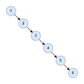
The average search time complexity of BST is O(logN), but in the worst case, it will be degraded to O(N). It happens when we insert the nodes one by one in order. For example, if we insert the elements in array [1, 2, 3, 4, 5, 6] into RST in order, what we get is as follows:
This kind of unbalanced BST is degraded to a single linked list. So the BST needs to keep balanced during the insert and delete of the node. That’s where the self-balancing binary search tree comes from.
Self-Balancing Binary Search Tree: it’s a binary search tree that automatically keeps its height small in the face of arbitrary item insertions and deletions. And the red-black tree is just one type of it.
Summary
As the first post of this series, I examined the background of the red-black tree bit by bit. I hope you can understand what’s self-balancing binary search tree and why we need it. In the next post, I will start to examine the behavior and property of the red-black tree.
Today, in this article I want to examine one concrete topic: how to delete a node from a binary search tree. This question is important for understanding other tree data structures, like the AVL tree, and the Red-Black tree.
As is common with many data structures, deletion is always the hardest operation. For example, to delete a specific element from the array, we need to shift all the elements after it by one index. And to delete one node from the linked list, we need to reset the pointer of the previous node (if it’s a doubled linked list, we need to reset more points, which is a more complex case). This is the same for the binary search tree as well. Let’s see in the following section.
Note: the idea of this article is inspired by the book Data Structures and Algorithm Analysis in C written by Mark Allen Weiss. The demo code shown in the following section is from this book. And I made some changes based on it. I highly recommend this great book to readers.
Deletion of the binary search tree
Before we can examine the deletion operation in depth, let’s quickly review the concept of the binary search tree as follows:
Binary search tree: is a binary tree holding the following property that for every node, X, in the tree, the values of all the keys in its left subtree are smaller than the key value in X, and the values of all the keys in its right subtree are larger than the key value in X.
Simply speaking, the binary search tree is a binary tree satisfying the binary search property. So each node of a binary search tree can have two children subtrees at most. When we need to delete one node from the binary search tree, then it’s necessary to consider the following 3 cases.
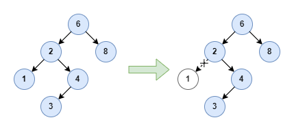
If the node is a leaf, then it can be deleted immediately. For example, to delete node 1 from the following binary search tree:
I will show you how to implement it at the code level later, which summarizes all the cases.
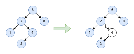
If the node has only one child subtree, the node can be deleted after we reset its parent’s pointer to bypass the node and point to its child node. For example, to delete node 4 as follows:
In the above example, node 4 has only one left child node 3. Let’s consider the symmetric scenario, imagine what will happen when it has only one right child node. The answer is it doesn’t influence how we handle the deleted node here and the result is the same. I will not draw the diagram here and leave it for you to explore.
The complicated case is how to deal with a node with two children. Before we introduce the solution, let’s clarify one concept about the binary search tree: successor:
Successor: is the node with the minimum value in the right subtree of any node.
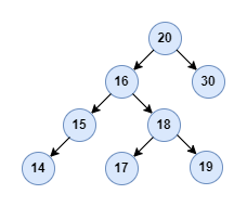
Let’s take node 16 in the above binary search tree as an example, the successor is node 17. All right! Based on this concept, the solution to delete a node with two children is straightforward:
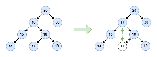
Replace the data of the deleted node with the value of the successor and recursively delete the successor from the right subtree.
Let’s try to analyze this solution. Firstly, replacing the data of the node with the value of the successor can keep the binary search property after the deletion operation. Secondly, since the successor has the minimum value of the subtree, which means it cannot have a left child. So the successor is either a leaf node without any child node or a node with only one right child node. So recursively deleting the successor can be resolved by the two simple cases we discussed above, it’s perfect, right? For instance, the deletion of node 16 goes as follows:
As we mentioned above, node 16‘s successor is node 17. So replace the value with 17 and delete node 17 from the right subtree, where node 17 is just a leaf node. Next, let’s implement the node deletion operation.
Code implementation
In this article, I will only show the codes related to the deletion operation rather than the complete implementation of a binary search tree. If you want to know how to write a BST from scratch, please refer to this GitHub repo.
Firstly, let’s examine the header file, which contains the data type definitions and function declarations.
BST delete(ET elem, BST T) { Position tmpCell; if (T == NULL) fatal("Element not found"); elseif (elem < T->Element) T->Left = delete(elem, T->Left); elseif (elem > T->Element) T->Right = delete(elem, T->Right); else// we found the element to be deleted if (T->Left != NULL && T->Right != NULL) // two children { tmpCell = findMinBST(T->Right); T->Element = tmpCell->Element; T->Right = delete(T->Element, T->Right); } else// one or zero children, change the pointer T pointing to new address(NULl or the child node) { tmpCell = T; // for leaf node, T will be reset to null if (T->Right == NULL) T = T->Left; elseif (T->Left == NULL) T = T->Right; free(tmpCell); } return T; }
Position findMinBST(BST T) { if (T == NULL) returnNULL; elseif (T->Left == NULL) return T; else return findMinBST(T->Left); }
I add some comments in the above code block which can help your understanding of this recursive algorithm. Please go ahead and think hard about it.
In the next section, we’ll have some open discussions about this solution. Let’s see whether there is any other solution. And what’re the potential issues of the current solution?
Open discussion
successor vs predecessor
Firstly, in the above solution, we delete the node with two children based on the successor. And there is the other concept called predecessor:
Predecessor: is the node with the maximum value in the left subtree of any node.
So similarly, the alternative solution to delete the node with two children is:
Replace the data of the deleted node with the value of the predecessor and recursively delete the predecessor from the left subtree.
We can do this by writing another helper function findMaxBST as follows:
1 2 3 4 5 6 7 8
Position findMaxBST(BST T) { if (T != NULL) while (T->Right != NULL) T = T->Right; return T; }
Does it work? The answer is yes. But the performance of the solution based on the predecessor is worse than the one based on the successor. Because the predecessor has the maximum value of the left subtree, it means that the predecessor can have two children. Then when we delete the predecessor recursively, the worst-case time complexity can reach O(logN) while the solution based on the successor only requires constant(O(1)) time. That’s the difference.
balanced vs unbalanced
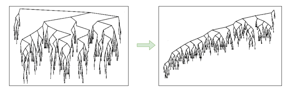
Although the above solution can work, it exposes a serious performance issue. The reason why people invent binary search tree data structures is that we can get O(logN) level performance for searching operations. But imagine what will happen if we keep inserting and deleting nodes in the binary search tree in the way we mentioned here. The depth of the tree will become unbalanced. The left subtree grows deeper than the right subtree because we are always replacing a deleted node with the successor(which is from the right subtree, right?)
The following image is borrowed from Mark’s great book I mentioned above, which clearly shows that the tree becomes unbalanced after many rounds of insertion and deletion. If you want to know about it in theory, please refer to the book.
For an unbalanced BST, the worst-case time complexity can be degraded to O(n). To keep the desired performance, people invent a more advanced data structure self-balancing binary search tree, like the AVL tree and Red-black tree. I will share about them in the coming articles, please keep watching my blog.
Summary
In this article, we examined various solutions to delete a node from the binary search tree and evaluated their performance. We also discussed some open questions about BST, which prove why we need more advanced data structures like the red-black tree.
In this last article, we examined how external mergesort works in theory, let’s implement it now.
First, you can find all the source codes of this implementation in this Github repo. In this repo, I implemented both two-way and multi-way solutions, which are tracked in different branches, please be aware of this. But for the sake of simplicity, I will focus on the generalized multi-way mergesort solution in this article.
Data Preparation
Before diving into the code, let’s define the problem we need to solve here. I will generate an input file containing several millions of seven digits random numbers, from 1,000,000 to 9,999,999. The random numbers can be duplicated, and each number is stored in one new line of the input file. The input file can be prepared with the following Bash script which calls GNU shuf :
1 2 3 4 5 6 7
#!/usr/bin/bash
# Author: Chris Bao # Generate millions of seven digits random integers # based on shuf utility
shuf -i 1000000-9999999 -n 7777777 > ./input.txt
The generated input file is roughly 60 MB in size. For modern computers, it can be loaded to memory easily. But since we are working external memory algorithm, so let’s assume we are running the algorithm on an old computer, which has only 100000 Byte memory. Based on this assumed restriction, we need to sort the numbers in the input file and save the result in a new file.
Implementation
Let’s define some global constants in this algorithm:
MEMORY_LIMIT denotes the 100000 bytes memory limit; In C, we can use the type unsigned int to store an integer in the range from 1,000,000 to 9,999,999. So RECORD_SIZE means each record(or integer) will take up 4 bytes of memory.
And by default, the algorithm will use the two-way merge, but the user can pass an argument to run a multi-way merge too.
Sort phase
The sort phase is implemented inside the separationSort function as follows:
// Reset memory buffer(zero-out the entire array) memset(buffer, 0, sizeof(unsignedint)*(MEMORY_LIMIT/RECORD_SIZE)); count = 0; fileNum++; buffer[count++] = (unsignedint)strtoul(line, NULL, 10); // add the current record into new buffer's as first element } }
// sort the last and final file mergeSort(buffer, count); char fileName[20]; sprintf(fileName, "./tmp/pass0/%d.txt", fileNum); if ((fp = fopen(fileName, "w+")) == NULL) { fprintf(stderr, "Failed to create file: %s.\n", fileName); exit(EXIT_FAILURE); } outputToFile(buffer, count, fp); free(buffer); free(line); printf("Sort phase done. %d tmp sorted files are produced.\n", fileNum); }
The logic is not difficult. The function takes the input file descriptor as a parameter and reads each line(via the getline method) in a loop until reaches the end of the file. The numbers will be read into the memory buffer before hitting the memory limit. When the memory buffer is full(100000 bytes), the numbers are sorted with the function mergeSort.
The function mergeSort is defined inside the file internal_sort.c, which implements the classic internal merge sorting algorithm. I will not cover it in this article, since you can find many documents about it online. If you don’t know about it, please spend some time learning about it. Of course, you can replace it with other sorting algorithms like quick sort too. I leave this for the readers.
After sorting, the numbers are saved in the temporary files in the directory of ./tmp/pass0. The filename is just the run number.
1 2 3 4 5 6 7 8 9 10 11
/* * Output sorted record to given file(of) * */
voidoutputToFile(unsignedint *buffer, int size, FILE *of) { int i; for (i = 0; i < size; i++) { fprintf(of, "%u\n", buffer[i]); } fclose(of); }
We can verify the result of the sort phase as follows:
You can see each file contains up to 25000 (equal to MEMORY_LIMIT/RECORD_SIZE) numbers and 312 files are created in pass0.
Note that I will not examine the details about how to make a new directory and how to open a new file to read or write. You can learn such Linux file I/O concepts by yourself.
Merge phase
The exMerge function controls the passes in the merge phase starting from pass1.
1 2 3 4 5 6 7 8 9 10 11 12 13 14
voidexMerge() { /* some code omitted ... */ int pass = 1; while (fileNum > 1) { exMergeSort(pass, fileNum); int remainer = fileNum % ways; fileNum = fileNum / ways; if (remainer > 0) { fileNum++; } pass++; } /* some code omitted ... */ }
The variable fileNum stores the run number in each pass. And the variable ways denotes the number of multi-way. Thus, the run number of the next pass should be calculated as fileNum / ways.
The detailed merging logic is inside the function exMergeSort, which takes two parameters. pass means the current pass number(starting from 1), while nums means how many runs(or sub-files) in the last pass need to be merged.
voidexMergeSort(int pass, int nums) { /* some code omitted ... */ int inputFileNum = 0; int run = 1; for (; inputFileNum < nums;) { // create the dir for current pass if (inputFileNum == 0) { int status; char dirName[20]; sprintf(dirName, "./tmp/pass%d", pass); if ((status = mkdir(dirName, S_IRWXU | S_IRWXU | S_IROTH | S_IXOTH)) == -1) { fprintf(stderr, "Failed to create tmp directory %s.\n", dirName); exit(EXIT_FAILURE); } } // open new file to merge in each run FILE *fm; char mergedFileName[20]; sprintf(mergedFileName, "./tmp/pass%d/%d.txt", pass, run); if ((fm = fopen(mergedFileName, "w+")) == NULL) { fprintf(stderr, "%s\n", strerror(errno)); fprintf(stderr, "merged file %s: can't create or open.\n", mergedFileName); } run++; /* some code omitted ... */ }
}
The above code creates a temp directory for each pass and a temp file for each run.
Next, we create an array of the input files for each run. And the input file is inside the temp directory of the last pass. Each run merges multiple files in the for loop. The only trick logic here is that the remaining files in the last run may be less than the number of ways declared, we need to handle that properly (line 5 of the below code block).
1 2 3 4 5 6 7 8 9 10 11 12 13 14 15 16
// Rewind the sorted files in previous pass, each run merge way_numbers numbers of files // Merge the sorted files with multi ways in N runs. // In the first N - 1 runs, each run merge ways numbers of files // In the last run, merge the remaining files. int way_numbers = run * ways <= nums ? ways : nums - inputFileNum; FILE *fiarr[way_numbers]; for (int i = 0; i < way_numbers; i++) { char inputFileName[20]; inputFileNum++; // start from 0 to nums sprintf(inputFileName, "./tmp/pass%d/%d.txt", pass - 1, inputFileNum); if ((fiarr[i] = fopen(inputFileName, "r")) == NULL) { fprintf(stderr, "%s\n", strerror(errno)); fprintf(stderr, "input file %s: can't create or open.\n", inputFileName); } rewind(fiarr[i]); }
Next, we need to read one number from every input file until only one file is not run out. Find the smallest one and save it in the temp output run file. And for the last remaining file, remember to put the rest numbers into the output file too.
// get and compare records until files runs out of records char *records[way_numbers]; for (int i = 0; i < way_numbers; i++) { records[i] = getRecord(fiarr[i]); } // loop until only one file is not run-out while(validateRecords(records, way_numbers )) { int index = getMinRecordIndex(records, way_numbers); fprintf(fm, "%s", records[index]); // print record to new merged file free(records[index]); // free the memory allocated by getline in getRecord function records[index] = getRecord(fiarr[index]); // Get new record from the file } // put the rest record in the last remaining file into new file int lastIndex = getLastRemainRecordIndex(records, way_numbers); while(records[lastIndex]) { fprintf(fm, "%s", records[lastIndex]); free(records[lastIndex]); records[lastIndex] = getRecord(fiarr[lastIndex]); }
The above code bock utilizes several methods like getRecord, validateRecords, getMinRecordIndex and getLastRemainRecordIndex as follows, and these functions are easy to understand.
/* * Returns a copy of the record * * */ char* getRecord(FILE *ifp) { char *line = NULL; size_t len = 0; ssize_t nread; while ((nread = getline(&line, &len, ifp)) != -1) { return line; } returnNULL; } /* * Validate whether at least two records are non-zero * */ boolvalidateRecords(char **records, int size) { int count = 0; for (int i = 0; i < size; i++) { if (records[i] != NULL) { count++; } } return count >= 2; }
/* * Get the min valid record's index * */ intgetMinRecordIndex(char **records, int size) { int index = 0; unsignedint min = (int)INFINITY; for (int i = 0; i < size; i++) { if (records[i] == NULL) { // pass invalid run-out record files continue; } if (strtoul(records[i], NULL, 10) < min) { min = strtoul(records[i], NULL, 10); index = i; } } return index; } /* * Get the last remainer of the records * */ intgetLastRemainRecordIndex(char **records, int size) { for (int i = 0; i < size; i++) { if (records[i] != NULL) { return i; } } }
In detail, you can refer to the source code of this github repo. Next, let’s evaluate the performance of this algorithm by tuning the number of ways for merging.
Performance Evaluation
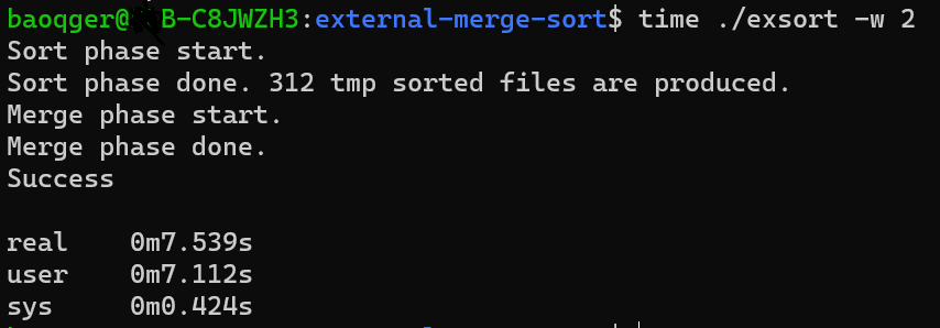
We’ll use the Linux time utility to measure the running time of this algorithm.
The result of two-way mergesort is:
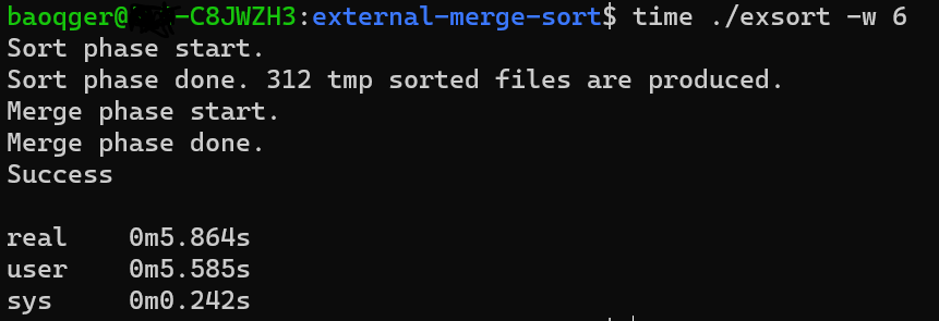
while six-way mergesort can complete with a shorter runtime.
This article will examine one interesting question which I came across when reading the book Programming Pearls. This question simply goes like this: How to sort a large disk file? The disk file has so much data that it cannot all fit into the main memory. I considered this algorithm question for a while; but noticed that all the classic sorting algorithms, like Quick sort and merge sort, can’t solve it easily. Then I did some research about it, and I will share what I learned in this article. I believe you can solve this problem as well, after reading this article.
Background of External Algorithm
Traditionally, computer scientists analyze the running time of an algorithm by counting the number of executed instructions, which is usually expressed as a function of the input size n, like the well-known Big O notation. This kind of algorithm complexity analysis is based on the Random access machine(RAM) model, which defines the following assumptions:
A machine with an unbounded amount of available memory;
Any desired memory location can be accessed in unit time;
Every instruction takes the same amount of time.
This model works well when the amount of memory that the algorithm needs to use is smaller than the amount of memory in the computer running the code.
But in the real world, some applications need to process data that are too large to fit into a computer’s main memory at once. And the algorithms used to solve such problems are called external memory algorithms or disk-based algorithms; since the input data are stored on an external memory storage device.
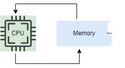
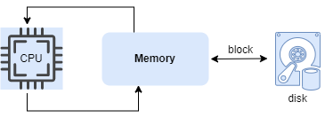
Instead of the RAM model, the external memory algorithm is analyzed based on the external memory model. The model consists of a CPU processor with an internal memory of bounded size, connected to an unbounded external memory. One I/O operation consists of moving a block of contiguous elements from external to internal memory(this is called page cache and is managed by the kernel.).
Compared with the main memory, the access speed of external memory is slower by several orders of magnitude, even though modern storage techniques such as SSD are already adopted. Thus, for external algorithms, the bottleneck of the performance is disk IO speed instead of the CPU cycles.
In this section, we examined the computational model of the external memory algorithms. Next, let’s review one typical type of external memory algorithm: external sorting.
External Mergesort
Similar to the traditional internal sorting algorithms, several different solutions are available for external sorting. In this article, I will focus on external mergesort.
External mergesort is a straightforward generalization of internal mergesort. The algorithm starts by repeatedly loading M input items into the memory(since the memory buffer size is limited, can only store M input items at once), sorting them, and writing them back out to disk. This step divides the input file into some(or many, if the input file is very large) sorted runs, each with M items sorted. Then the algorithm repeatedly merges multiple sorted runs, until only a single sorted run containing all the input data remains.
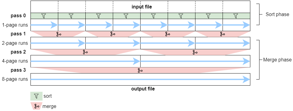
Let’s use the following example model to analyze this algorithm. First of all, assume the memory buffer is limited, and the size is one page. And the input file size is 8 pages. External mergesort can be divided into two phases: sort phase and merge phase.
Sort phase:
Divide the entire input file into 8 groups, each group size is one page(memory buffer capacity).
Load each page into the memory, sort the items in the memory buffer(with an internal sorting algorithm), and save the sorted items in a temporary sub-file. Each sub-file is called a run.
At the end of the sort phase, 8 temporary sorted 1-page runs will be created. This step can be marked as pass 0.
Merge phase:
The 8 sorted runs in pass 0 will be merged into a single sorted file with 3 more passes.
pass 1: Perform 4 runs for the merge.
Run 1: Merge the first two small 1-page runs into a big 2-page run. This merging step goes as follows:
Read the first two sorted sub-files (one item from each file).
Find the smaller item, output it in the new sub-file, and the appropriate input sub-file is advanced. Repeat this cycle until the input sub-file is completed. This routine’s logic is the same as the internal mergesort algorithm.
Run 2: Merge the next two 1-page runs into a 2-page run.
Run 3 and 4: follow the same process.
At the end of pass 1, 4 temporary sorted 2-page runs will be created.
pass 2: Perform 2 runs for the merge.
At the end of pass 2, 2 temporary sorted 4-page runs will be created.
pass 3: Perform 1 run for the merge.
At the end of pass 3, the final 8-page run containing all the sorted items will be created.
Note: the above process may seem complicated at the first sight, but the logic is nearly the same as the internal merge sort. The only difference is internal merging is based on memory buffers, while external merging is based on disk files, and needs reading the item from disk to memory.
Since we keep merging two small sub-files into a big one with doubled size, the above algorithm can be called two-way external merge sorting. We can generalize the idea to multi-way external merge sorting, which merges M runs into one.
Next, let’s analyze its complexity. Suppose the input file has N items and each page consists of B items. And M denotes the number of ways used in the merge phase, thus the number of passes should be: logM(N/B) + 1, where plus one means the first pass in the sort phase. And each pass, each item is read and written once from and to the disk file. So the total number of disk I/O is: 2N*(logM(N/B) + 1)
Summary
In this article, we examined the abstract computational model of the external memory algorithm and analyzed the details of the external mergesort algorithm. Next article, let’s implement the code and evaluate the performance.
In the last article, we investigated how the allocated chunks are aligned and stored in the heap. This article continues to examine how to free a chunk of memory and how the freed chunks are stored in the heap.
Hands-on demo
Let’s continue debugging the demo code shown in the last article:
Previously, we allocated a chunk of memory and put data in it. The next line will free this chunk. Before we run the instruction and show the demo result, let’s discuss the theory first.
The freed chunk will not be returned to the kernel immediately after the free is called. Instead, the heap allocator keeps track of the freed chunks in a linked list data structure. So the freed chunks in the linked list can be reused when the application requests new allocations again. This can decrease the performance overhead by avoiding too many system calls.
The allocator could store all the freed chunks together in a long linked list, this would work but the performance would be slow. Instead, the glibc maintains a series of freed linked lists called bins, which can speed up the allocations and frees. We will examine how bins work later.
It is worth noting that each free chunk needs to store pointers to other chunks to form the linked list. That’s what we discussed in the last section, there’re two points in the malloc_chunk structure: fd and bk, right? Since the user data region of the freed chunk is free for use by the allocator, so it repurposes the user data region as the place to store the pointer.
Based on the above description, the following picture illustrates the exact structure of a freed chunk:
1 2 3 4 5 6 7 8 9 10 11 12 13 14 15
chunk-> +-+-+-+-+-+-+-+-+-+-+-+-+-+-+-+-+-+-+-+-+-+-+-+-+-+-+-+-+-+-+-+-+ | Size of previous chunk, if freed | +-+-+-+-+-+-+-+-+-+-+-+-+-+-+-+-+-+-+-+-+-+-+-+-+-+-+-+-+-+-+-+-+ | Size of chunk, in bytes |A|M|P| mem-> +-+-+-+-+-+-+-+-+-+-+-+-+-+-+-+-+-+-+-+-+-+-+-+-+-+-+-+-+-+-+-+-+ | pointer to the next freed chunk | +-+-+-+-+-+-+-+-+-+-+-+-+-+-+-+-+-+-+-+-+-+-+-+-+-+-+-+-+-+-+-+-+ | pointer to the previous freed chunk | +-+-+-+-+-+-+-+-+-+-+-+-+-+-+-+-+-+-+-+-+-+-+-+-+-+-+-+-+-+-+-+-+ . . . ...... . nextchunk-> +-+-+-+-+-+-+-+-+-+-+-+-+-+-+-+-+-+-+-+-+-+-+-+-+-+-+-+-+-+-+-+-+ | Size of chunk | +-+-+-+-+-+-+-+-+-+-+-+-+-+-+-+-+-+-+-+-+-+-+-+-+-+-+-+-+-+-+-+-+
Now step over one line in gdb and check chunks in the heap as follows:
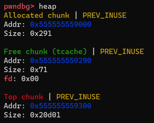
You can see the changes: the allocated chunk is marked as a Free chunk (tcache) and pointer fd is set(which indicates this freed chunk is inserted into a linked list).
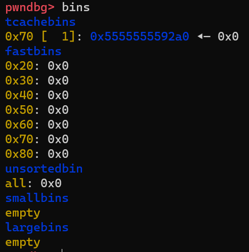
The tcache is one kind of bins provided by glibc. The gdb pwndbg plugin allows you to check the content of bins by running command bins as follows:
Note that the freed chunk(at 0x5555555592a0) is inserted into tcache bins as the liked list header.
Note that there 5 types of bins: small bins, large bins, unsorted bins, fast bins and tcache bins. If you don’t know, don’t worry I will examine them in the following section.
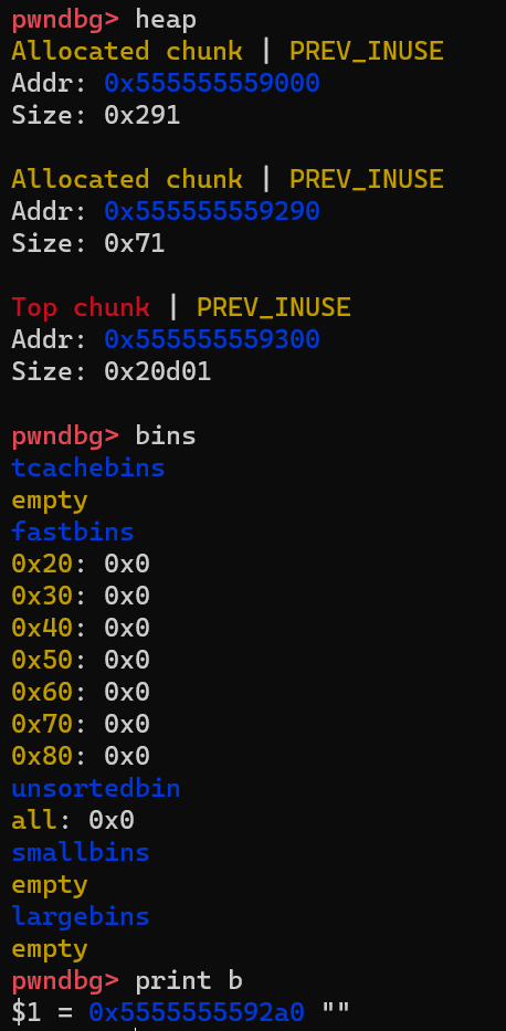
According to the definition, after the second malloc(100) is called, the allocator should reuse the freed chunk in the bins. The following image can prove this:
The freed chunk at 0x555555559290 is in use again and all bins are empty after the chunk is removed from the linked list. All right!
Recycling memory with bins
Next, I want to spend a little bit of time examining why we need bins and how bins optimize chunk allocation and free.
If the allocator keeps track of all the freed chunks in a long linked list. The time complexity is O(N) for the allocator to find a freed chunk with fit size by traversing from the head to the tail. If the allocator wants to keep the chunks in order, then at least O(NlogN) time is needed to sort the list by size. This slow process would have a bad impact on the overall performance of programs. That’s the reason why we need bins to optimize this process. In summary, the optimization is done on the following two aspects:
High-performance data structure
Per-thread cache without lock contention
High-performance data structure
Take the small bins and large bins as a reference, they are defined as follows:
1 2 3 4 5
#define NBINS 128
typedefstructmalloc_chunk* mchunkptr;
mchunkptr bins[NBINS * 2 - 2];
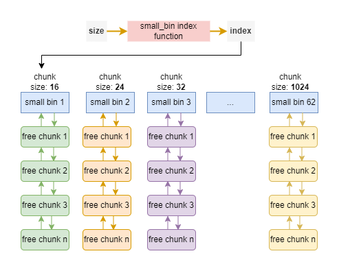
They are defined together in an array of linked lists and each linked list(or bin) stores chunks that are all the same fixed size. From bins[2] to bins[63] are the small bins, which track freed chunks less than 1024 bytes while the large bins are for bigger chunks. small bins and large bins can be represented as a double-linked list shown below:
The glibc provides a function to calculate the index of the corresponding small(or large) bin in the array based on the requested size. Since the index operation of the array is in O(1) time. Moreover, each bin contains chunks of the same size, so it can also take O(1) time to insert or remove one chunk into or from the list. As a result, the entire allocation time is optimized to O(1).
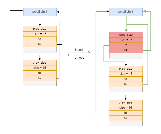
bins are LIFO(Last In First Out) data structure. The insert and remove operations can be illustrated as follows:
Moreover, for small bins and large bins, if the neighbors of the current chunk are free, they are merged into a larger one. That’s the reason we need a double-linked list to allow running fast traverse both forward and backward.
Unlike small bins and large bins, fast bins and tcache bins chunks are never merged with their neighbors. In practice, the glibc allocator doesn’t set the P special flag at the start of the next chunk. This can avoid the overhead of merging chunks so that the freed chunk can be immediately reused if the same size chunk is requested. Moreover, since fast bins and tcache bins are never merged, they are implemented as a single-linked list.
This can be proved by running the second free method in the demo code and checking the chunks in the heap as follows:
First, the top chunk’s size is still 0x20d01 rather than 0x20d00, which indicates the P bit is equal to 1. Second, the Free chunk only has one pointer: fd. If it’s in a double-linked list, both fd and bk should point to a valid address.
Per-thread cache without lock contention
The letter t in tcache bins represents the thread, which is used to optimize the performance of multi-thread programs. In multi-thread programming, the most common way solution to prevent the race condition issue is using the lock or mutex. Similarly, The glibc maintains a lock in the data structure for each heap. But this design comes with a performance cost: lock contention, which happens when one thread attempts to acquire a lock held by another thread. This means the thread can’t do any tasks.
tcache bins are per-thread bins. This means if the thread has a chunk on its tcache bins, it can serve the allocation without waiting for the heap lock!
Summary
In this article, we examined how the userland heap allocaor works by debugging into the heap memory with gdb. The discussion is fully based on the glibc implementation. The design and behavior of the glibc heap allocator are complex but interesting, what we covered here just touches the tip of the iceberg. You can explore more by yourself.
Moreover, I plan to write a simple version of a heap allocator for learning and teaching purpose. Please keep watching my blog!
The previous article gave a general overview of memory management. The story goes on. In this section, let’s break into the heap memory to see how it works basically.
Memory allocator
We need to first understand some terminology in the memory management field:
mutator: the program that modifies the objects in the heap, which is simply the user application. But I will use the term mutator in this article.
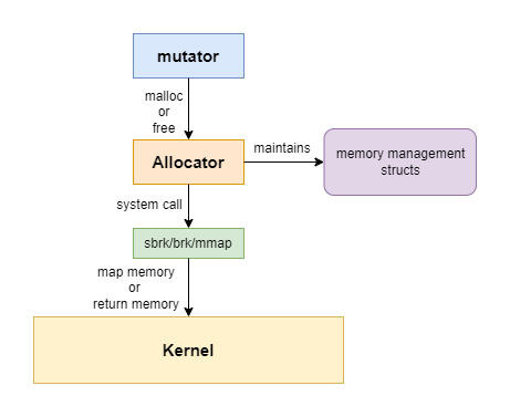
allocator: the mutator doesn’t allocate memory by itself, it delegates this generic job to the allocator. At the code level, the allocator is generally implemented as a library. The detailed allocation behavior is fully determined by the implementations, in this article I will focus on the memory allocator in the library of glibc.
The relationship between the mutator and allocator is shown in the following diagram:
There is a third component in the memory management field: the garbage collector(GC). GC reclaims memories automatically. Since this article is talking about manual heap memory allocation in system programming, we will ignore GC for now. GC is a very interesting technical challenge, I will examine it in the future. Please keep watching my blog!
Hands-on demo
We will use gdb and pwndbg(which is a gdb plugin) and break into the heap memory to see how it works. The gdb provides the functionality to extend it via Python plugins. pwndbg is the most widely used.
The demo code above just allocates some memory, set the content of the memory and releases it later. And then allocate other chunks of memory again. Very simple, all right?
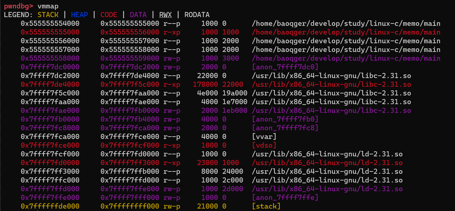
First, set a breakpoint at line 7(the first malloc call) and run the program in gdb. Then run vmmap command from pwndbg, which can get the process memory layout as follows:
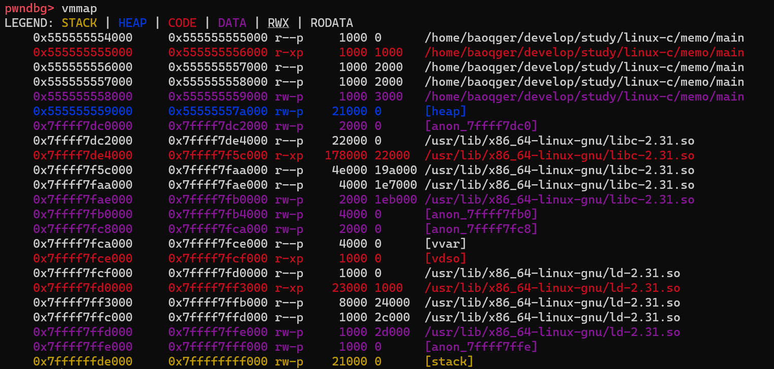
Note that there is no heap segment yet before the first malloc call is made. After step over one line in gdb, check the layout again:
Now the heap segment is created with the size of 132KB(21000 in hexadecimal). As described above, the kernel maps 132KB of physical memory to this process’s virtual memory and marks this 132KB block of physical memory as used to isolate other processes. This mapping routine is done via system calls like brk, sbrk and mmap. Please investigate these system calls yourself.
132KB is much bigger than the 100B(the size passed to malloc). This behavior can answer one question at the beginning of this article. The system calls aren’t necessary to be triggered each time when malloc is called. This design is aimed to decrease performance overhead. Now the 132KB heap memory is maintained by the allocator. Next time the application calls malloc again, the allocator will allocate memory for it.
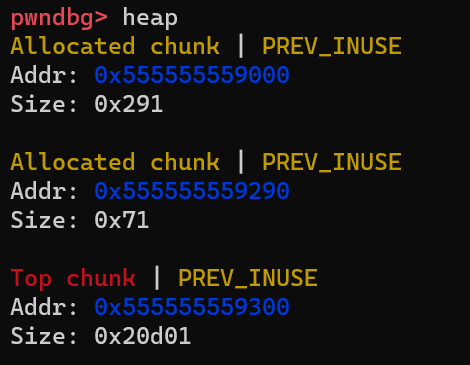
Next, step one more line in gdb to assign value(“AAAABBBBCCCCDDDD”) to the allocated block. Let’s check the content of this 132KB heap segment with heap command as follows:
There are 3 chunks. Let’s examine these chunks one by one.
The top chunk contains all the remaining memories which have not been allocated yet. In our case, the kernel maps 132KB of physical memory to this process. And 100B memory is allocated by calling malloc(100), so the remaining memories are in the top chunk. The top chunk stays on the border of the heap segment, and it can grow and shrink as the process allocates more memory or release unused memory.
Then let’s look at the chunk with the size of 0x291. The allocator uses this chunk to store heap management structures. It is not important for our analysis, just skip it.
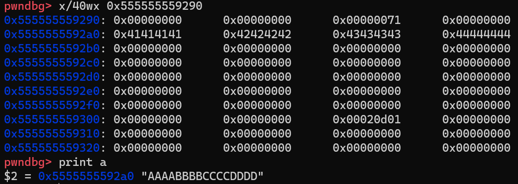
What we care about is the chunk in the middle with a size of 0x71. It should be the block we requested and contains the string “AAAABBBBCCCCDDDD”. We can verify this point by checking its content:
gdb’s x command can display the memory contents at a given address using the specified format. x/40wx 0x555555559290 prints 40 words(each word is 32 bits) of memories starting from 0x555555559290 in the hexadecimal format.
We can see that the string “AAAABBBBCCCCDDDD” is there. So our guess is correct. But the question is why the size of this chunk is 0x71. To understand this, we need to first analyze how the allocator stores chunk. A chunk of memory is represented by the following structure:
1 2 3 4 5 6 7 8
structmalloc_chunk { INTERNAL_SIZE_T prev_size; /* Size of previous chunk (only if free). */ INTERNAL_SIZE_T size; /* Size in bytes, including overhead. */ structmalloc_chunk* fd;/* double links -- used only if free. */ structmalloc_chunk* bk;/* double links -- used only if free. */ };
typedefstructmalloc_chunk* mchunkptr;
prev_size: the size of the previous chunk only when the previous chunk is free, otherwise when the previous chunk is in use it stores the user data of the previous chunk.
size: the size of the current chunk.
fd: pointer to the next free chunk only when the current chunk is free, otherwise when the current chunk is in use it stores the user data.
bk: pointer to the previous free chunk. Behaves in the same way as pointer fd.
Based on the above description, the following picture illustrates the exact structure of an allocated chunk:
1 2 3 4 5 6 7 8 9 10 11 12
chunk-> +-+-+-+-+-+-+-+-+-+-+-+-+-+-+-+-+-+-+-+-+-+-+-+-+-+-+-+-+-+-+-+-+ | Size of previous chunk, if freed | +-+-+-+-+-+-+-+-+-+-+-+-+-+-+-+-+-+-+-+-+-+-+-+-+-+-+-+-+-+-+-+-+ | Size of chunk, in bytes |A|M|P| mem-> +-+-+-+-+-+-+-+-+-+-+-+-+-+-+-+-+-+-+-+-+-+-+-+-+-+-+-+-+-+-+-+-+ | User data starts here... . . . . . . | nextchunk-> +-+-+-+-+-+-+-+-+-+-+-+-+-+-+-+-+-+-+-+-+-+-+-+-+-+-+-+-+-+-+-+-+ | Size of chunk | +-+-+-+-+-+-+-+-+-+-+-+-+-+-+-+-+-+-+-+-+-+-+-+-+-+-+-+-+-+-+-+-+
chunk: indicates the real starting address of the object in the heap memory.
mem: indicates the returned address by malloc.
The memory in between is reserved for the metadata mentioned above: prev_size and size. On a 64-bit system, they’re (type of INTERNAL_SIZE_T) 8 bytes in length.
For the size field, it is worth noting:
It includes both the size of metadata and the size of the actual user data.
It is usually aligned to a multiple of 16 bytes. You can investigate the purpose of memory alignment by yourself.
It contains three special flags(A|M|P) at the three least significant bits. We can ignore the other two bits for now, but the last bit indicates whether the previous chunk is in use(set to 1) or not(set to 0).
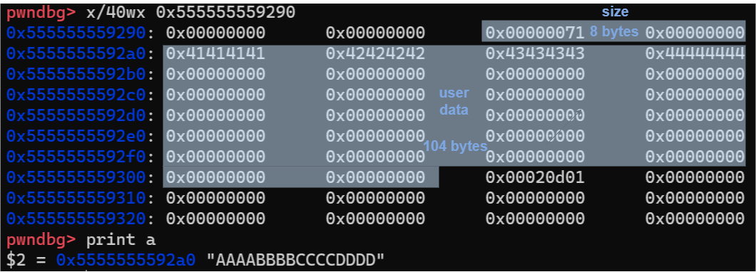
According to this, let’s review the content of this chunk again:
I add marks on the image to help you understand. Let’s do some simple calculations. 100 + 8 = 108, 100 is the size of memory we requested, 8 is the size of metadata(for size field). Then 108 is aligned to 112 as a multiple of 16 bytes. Finally, since the special flag P is set to 1, then we get 112 + 1 = 113(0x71)(that’s the reason why the size is 0x71 instead of 0x70).
In this section, we break into the heap segment and see how an allocated chunk works. Next, we’ll check how to free a chunk.
In my eyes, compared with developing applications with high-level programming languages, one of the biggest differences for system programming with low-level languages like C and C++, is you have to manage the memory by yourself. So you call APIs like malloc, and free to allocate the memory based on your need and release the memory when the resource is no longer needed. It is not only one of the most frequent causes of bugs in system programming; but also can lead to many security issues.
It’s not difficult to understand the correct usage of APIs like malloc, and free. But have you ever wondered how they work, for example:
When you call malloc, does it trigger system calls and delegate the task to the kernel or there are some other mechanisms?
When you call malloc(10) and try to allocate 10 bytes of heap memory, how many bytes of memory do you get? 10 bytes or more?
When the memory is allocated, where exactly the heap objects are located?
When you call free, is the memory directly returned to the kernel?
This article will try to answer these questions.
Note that memory is a super complex topic, so I can’t cover everything about it in one article (In fact, what is covered in this article is very limited). This article will focus on userland memory(heap) allocation.
Process memory management overview
Process virtual memory
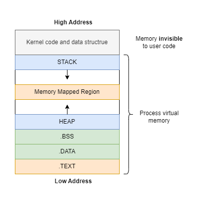
Every time we start a program, a memory area for that program is reserved, and that’s process virtual memory as shown in the following image:
You can note that each process has one invisible memory segment containing kernel codes and data structures. This invisible memory segment is important; since it’s directly related to virtual memory, which is employed by the kernel for memory management. Before we dive into the other different segments, let’s understand virtual memory first.
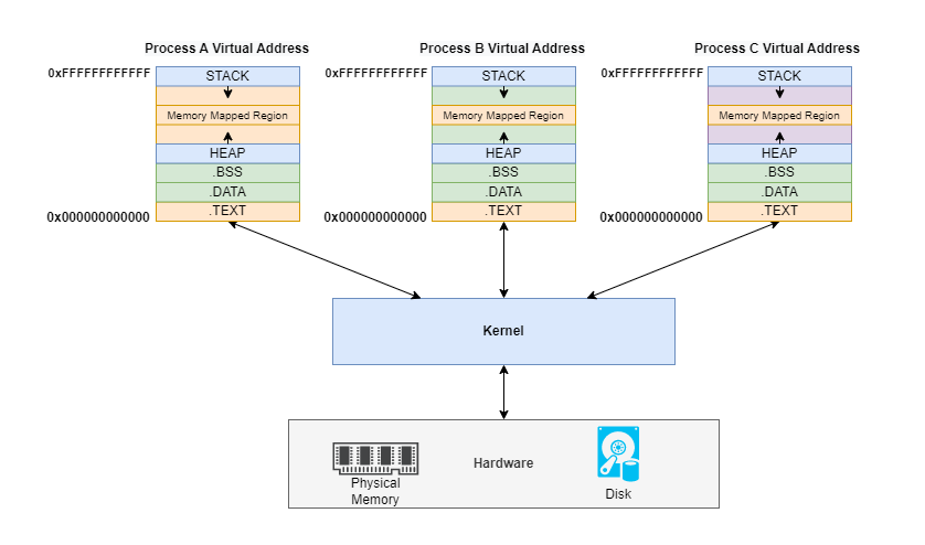
Virtual memory technique
Why do we need virtual memory? Virtual memory is a service provided by the kernel in the form of abstraction. Without virtual memory, applications would need to manage their physical memory space, coordinating with every other process running on the computer. Virtual memory leaves that management to the kernel by creating the maps that allow translation between virtual and physical memory. The kernel creates an illusion that each process occupies the entire physical memory space. We can also realize process isolation based on virtual memory to enhance security.
Virtual memory is out of this article’s scope, if you’re interested, please take a look at the core techniques: paging and swapping.
Static vs Dynamic memory allocation
Next, let’s take a close look at the process memory layout above and understand where they are from. Generally speaking, there are two ways via which memories can be allocated for storing data: static and dynamic. Static memory allocation happens at compile time, while dynamic memory allocation occurs at runtime.
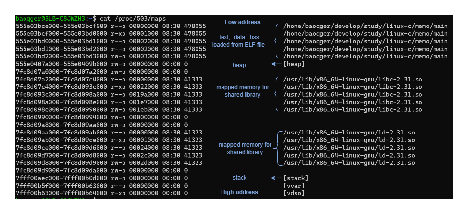
When a program started, the executable file(on the Linux system, it’s called an ELF file) will be loaded into the memory as a Process Image. This ELF file contains the following segments:
.TEXT: contains the executable part of the program with all the machine codes.
.DATA: contains initialized static and global variables.
.BSS: is short for block started by symbol contains uninitialized static and global variables.
The ELF file will be loaded by the kernel and create a process image. And these static data will be mapped into the corresponding segments of the virtual memory. The ELF loader is also an interesting topic, I will write another article about it in the future. Please keep watching my blog!
The memory-mapped region segment is used for storing the shared libraries.
Finally, stack and heap segments are produced at runtime dynamically, which are used to store and operate on temporary variables that are used during the execution of the program. Previously, I once wrote an article about the stack, please refer to it if you want to know the details.
The only remaining segment we didn’t mention yet is the heap, which is this article’s focus!
You can check the memory layout of one process by examining this file /proc/{pid}/maps as below:
Note that the above investigation doesn’t consider multiple threads. The memory layout of the process with multi-threads will be more complex, please refer to other online documents.
In this section, we had a rough overview of memory management from top to bottom. Hope you can see the big picture and know where we are. Next, let’s dig into the heap segment and see how it works.
In this post, I want to introduce my new project: cPacketSniffer. I worked on it for the past two months. Finally, I worked it out and feel very proud of putting it here!
Motivation
Simply speaking, I want to sharpen my techniques in network programming and Linux system programming. Both of these two topics can lead you to the bottom of computers or software. Feynman said “There is plenty of room at the bottom”, I think this physics law can apply to software as well.
Acknowledgement
It’s very lucky for me to come across this site “Network programming in Linux”, which developed a network packet capturing tool with C++. After confirming that the documents and source code on this site is completed and clear, I decided to refactor it with C language. That’s the starting point for my project cPacketSniffer.
Features
As a network packets sniffer, cPacketSniffer provides the following features:
Integrate with libpcap to support: filtering captured packets, capturing packets offline, capturing packets on specific devices and capturing packets in promiscuous mode.
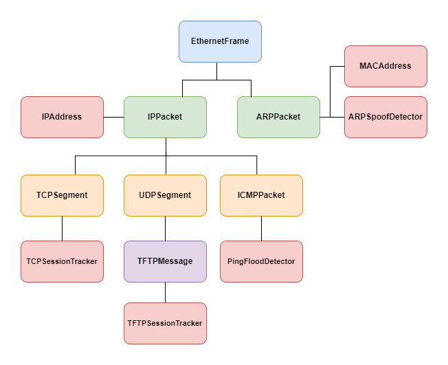
Analyze network packets at low layers of TCP/IP stack, including Ethernet, ARP, ICMP, IP(IPv4), TCP, UDP, etc. Also one protocol in the application layer: TFTP.
Detect network security attacks:
ARP spoofing detection.
Ping flood detection.
Analyze and track network traffics:
TCP session tracking and traffic analysis.
TFTP session tracking and traffic analysis.
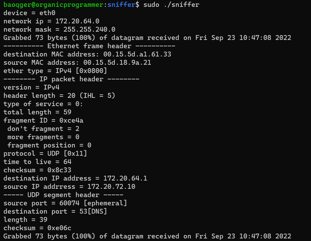
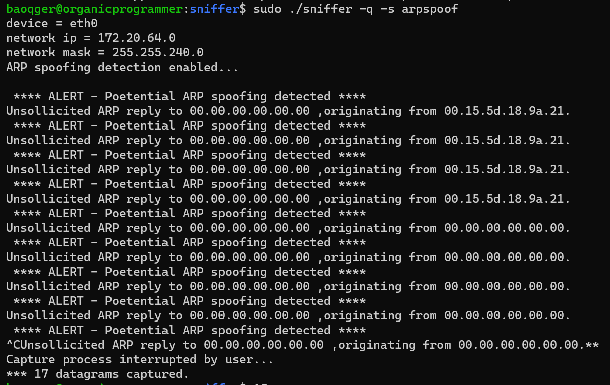
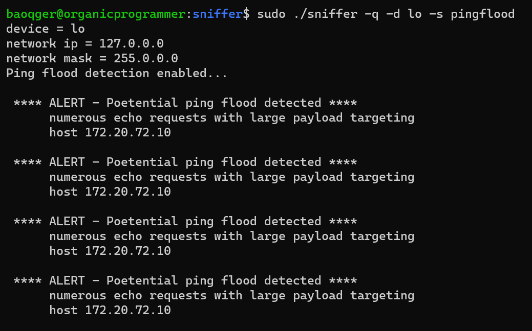
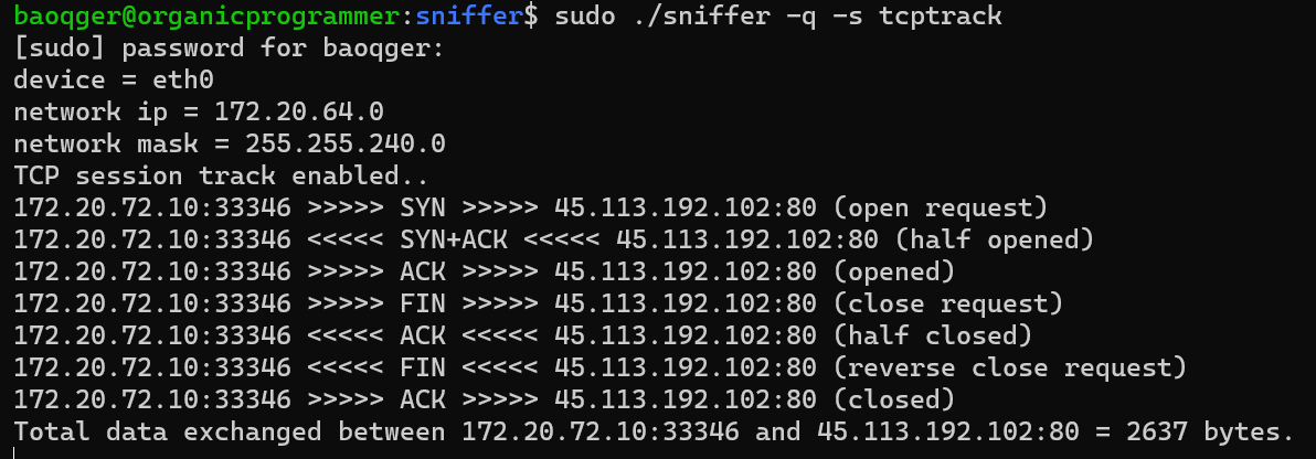
The following images demonstrate some typical usages of cPacketSniffer:
Packet Analysis:
ARP Spoofing Detection:
PING Flood Detection:
TCP Session Tracking:
Besides the above network programming-related functionalities, it also covers the following points:
Develop a generic data structure in C.
Error handling in C.
Data encapsulation (object-oriented style programming) in C.
Manual memory management in C.
etc.
This article will not cover these points in detail, I will write articles on these topics separately in the future. Please keep watching my blog!
Future work
Now cPacketSniffer can work as a network packet sniffer based on the design. Moreover, it can also serve as a testbed to try experimental features. Next step I plan to try the following ideas:
Implement the network intrusion detection function.
Improve the performance with advanced data structures, like binary search trees.
Memory and cache performance tuning.
Automatic memory management by Garbage Collection.
In the previous article, we examined how to write a Kernel module and load it dynamically into a running Linux system. Based on this understanding, let’s continue our journey to write a Netfilter module as our mini-firewall.
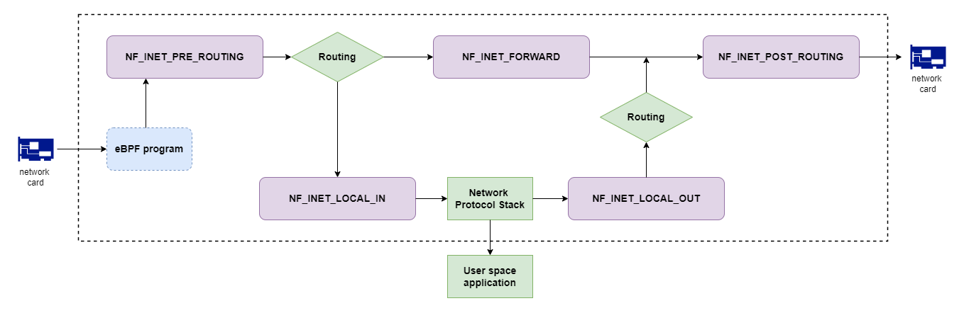
Netfilter architecture.
Basics of Netfilter hooks
The Netfilter framework provides a bunch of hooks in the Linux kernel. As network packets pass through the protocol stack in the kernel, they will traverse these hooks as well. And Netfilter allows you to write modules and register callback functions with these hooks. When the hooks are triggered, the callback functions will be called. This is the basic idea behind Netfilter architecture. Not difficult to understand, right?
Currently, Netfilter provides the following 5 hooks for IPv4:
NF_INET_PRE_ROUTING: is triggered right after the packet has been received on a network card. This hook is triggered before the routing decision was made. Then the kernel determines whether this packet is destined for the current host or not. Based on the condition, the following two hooks will be triggered.
NF_INET_LOCAL_IN: is triggered for network packets that are destined for the current host.
NF_INET_FORWARD: is triggered for network packets that should be forwarded.
NF_INET_POST_ROUTING: is triggered for network packets that have been routed and before being sent out to the network card.
NF_INET_LOCAL_OUT: is triggered for network packets generated by the processes on the current host.
The hook function you defined in the module can mangle or filter the packets, but it eventually must return a status code to Netfilter. There are several possible values for the code, but for now, you only need to understand two of them:
NF_ACCEPT: this means the hook function accepts the packet and it can go on the network stack trip.
NF_DROP: this means the packet is dropped and no further parts of the network stack will be traversed.
Netfilter allows you to register multiple callback functions to the same hook with different priorities. If the first hook function accepts the packet, then the packet will be passed to the next functions with low priority. If the packet is dropped by one callback function, then the next functions(if existing) will not be traversed.
As you see, Netfilter has a big scope and I can’t cover every detail in the articles. So the mini-firewall developed here will work on the hook NF_INET_PRE_ROUTING, which means it works by controlling the inbound network traffic. But the way of registering the hook and handling the packet can be applied to all other hooks.
Note: there is another remarkable question: what’s the difference between Netfilter and eBPF? If you don’t know eBPF, please refer to my previous article. Both of them are important network features in the Linux kernel. The important thing is Netfilter and eBPF hooks are located in different layers of the Kernel. As I drew in the above diagram, eBPF is located in a lower layer.
Kernel code of Netfilter hooks
To have a clear understanding of how the Netfilter framework is implemented inside the protocol stack, let’s dig a little bit deeper and take a look at the kernel source code (Don’t worry, only shows several simple functions). Let’s use the hook NF_INET_PRE_ROUTING as an example; since the mini-firewall will be written based on it.
When an IPv4 packet is received, its handler function ip_rcv will be called as follows:
skb = ip_rcv_core(skb, net); if (skb == NULL) return NET_RX_DROP; // run Netfilter NF_INET_PRE_ROUTING hook's callback function return NF_HOOK(NFPROTO_IPV4, NF_INET_PRE_ROUTING, net, NULL, skb, dev, NULL, ip_rcv_finish); }
In this handler function, you can see the hook is passed to the function NF_HOOK. Based on the name NF_HOOK, you can guess that it is for triggering the Netfilter hooks. Right? Let’s continue to examine how NF_HOOK is implemented as follows:
//In source code file /kernel-src/include/linux/netfilter.h staticinlineint NF_HOOK(uint8_t pf, unsignedint hook, struct net *net, struct sock *sk, struct sk_buff *skb, struct net_device *in, struct net_device *out, int (*okfn)(struct net *, struct sock *, struct sk_buff *)) { int ret = nf_hook(pf, hook, net, sk, skb, in, out, okfn); if (ret == 1) ret = okfn(net, sk, skb); // in our case: okfn is ip_rcv_finish return ret; } /** * nf_hook - call a netfilter hook * * Returns 1 if the hook has allowed the packet to pass. The function * okfn must be invoked by the caller in this case. Any other return * value indicates the packet has been consumed by the hook. */ staticinlineintnf_hook(u_int8_t pf, unsignedint hook, struct net *net, struct sock *sk, struct sk_buff *skb, struct net_device *indev, struct net_device *outdev, int (*okfn)(struct net *, struct sock *, struct sk_buff *)) { // code omit }
The function NF_HOOK contains two steps:
First, runs the hook’s callback functions by calling the underlying function nf_hook.
Second, invokes the function okfn (passed to NF_HOOK as the argument), if the packet passes through the hook functions and doesn’t drop.
For the hook NF_INET_LOCAL_IN, the function ip_rcv_finish will be invoked after the hook functions pass. Its job is to pass the packet on to the next protocol handler(TCP or UDP) in the protocol stack to continue its journey!
The other 4 hooks all use the same function NF_HOOK to trigger the callback functions. The following table shows where the hooks are embedded in the kernel, I leave them to the readers.
Hook
File
Function
NF_INET_PRE_ROUTING
/kernel-src/net/ipv4/ip_input.c
ip_rcv()
NF_INET_LOCAL_IN
/kernel-src/net/ipv4/ip_input.c
ip_local_deliver()
NF_INET_FORWARD
/kernel-src/net/ipv4/ip_forward.c
ip_forward()
NF_INET_POST_ROUTING
/kernel-src/net/ipv4/ip_output.c
ip_build_and_send_pkt()
NF_INET_LOCAL_OUT
/kernel-src/net/ipv4/ip_output.c
ip_output()
Next, Let’s review the Netfilter’s APIs to create and register the hook function.
Netfilter API
It’s straightforward to create a Netfilter module, which involves three steps:
Define the hook function.
Register the hook function in the kernel module initialization process.
Unregister the hook function in the kernel module clean-up process.
Let’s go through them quickly one by one.
Define a hook function
The hook function name can be whatever you want, but it must follow the signature below:
The hook function can mangle or filter the packet whose data is stored in the sk_buff structure (we can ignore the other two parameters; since we don’t use them in our mini-firewall). As we mentioned above, the callback function must return a Netfilter status code which is an integer. For instance, the accepted and dropped status is defined as follows:
1 2 3 4
// In source code file /kernel-src/include/uapi/linux/netfilter.h /* Responses from hook functions. */ #define NF_DROP 0 #define NF_ACCEPT 1
Register and unregister a hook function
To register a hook function, we should wrap the defined hook function with related information, such as which hook you want to bind to, the protocol family and the priority of the hook function, into a structure struct nf_hook_ops and pass it to the function nf_register_net_hook.
1 2 3 4 5 6 7 8 9 10 11
//In source code file /kernel-src/include/linux/netfilter.h structnf_hook_ops { /* User fills in from here down. */ nf_hookfn *hook; // callback function structnet_device *dev;// network device interface void *priv; u_int8_t pf; // protocol unsignedint hooknum; // Netfilter hook enum /* Hooks are ordered in ascending priority. */ int priority; // priority of callback function };
Most of the fields are very straightforward to understand. The one need to emphasize is the field hooknum, which is just the Netfilter hooks discussed above. They are defined as enumerators as follows:
Next, let’s take a look at the functions to register and unregister hook functions goes as follows:
1 2 3 4
//In source code file /kernel-src/include/linux/netfilter.h /* Function to register/unregister hook points. */ intnf_register_net_hook(struct net *net, conststruct nf_hook_ops *ops); voidnf_unregister_net_hook(struct net *net, conststruct nf_hook_ops *ops);
The first parameter struct net is related to the network namespace, we can ignore it for now and use a default value.
Next, let’s implement our mini-firewall based on these APIs. All right?
Implement mini-firewall
First, we need to clarify the requirements for our mini-firewall. We’ll implement two network traffic control rules in the mini-firewall as follows:
Network protocol rule: drops the ICMP protocol packets.
IP address rule: drops the packets from one specific IP address.
The completed code implementation is in this Github repo.
Drop ICMP protocol packets
ICMP is a network protocol widely used in the real world. The popular diagnostic tools like ping and traceroute run the ICMP protocol. We can filter out the ICMP packets based on the protocol type in the IP headers with the following hook function:
The logic in the above hook function is easy to understand. First, we retrieve the IP headers from the network packet. And then according to the protocol type field in the headers, we decided to accept TCP and UDP packets but drop the ICMP packets. The only technique we need to pay attention to is the function ip_hdr, which is the kernel function defined as follows:
The function ip_hdr delegates the task to the function skb_network_header. It gets IP headers based on the following two data:
head: is the pointer to the packet;
network_header: is the offset between the pointer to the packet and the pointer to the network layer protocol header. In detail, you can refer to this document.
Next, we can register the above hook function as follows:
Next, let’s try to ban the traffic from this IP address.
Drop packets source from one specific IP address
As we mentioned above, multiple callback functions are allowed to be registered on the same Netfilter hook. So we will define the second hook function with a different priority. The logic of this hook function goes like this: we can get the source IP address from the IP headers and make the drop or accept decision according to it. The code goes as follows
sb = skb; iph = ip_hdr(sb); sip = ntohl(iph->saddr); // get source ip address; sprintf(str, "%u.%u.%u.%u", IPADDRESS(sip)); // convert to standard IP address format if(!strcmp(str, ip_addr_rule)) { return NF_DROP; } else { return NF_ACCEPT; } } }
This hook function uses two interesting techniques:
ntohl: is a kernel function, which is used to convert the value from network byte order to host byte order. Byte order is related to the computer science concept of Endianness. Endianness defines the order or sequence of bytes of a word of digital data in computer memory. A big-endian system stores the most significant byte of a word at the smallest memory address. A little-endian system, in contrast, stores the least-significant byte at the smallest address. Network protocol uses the big-endian system. But different OS and platforms run various Endianness system. So it may need such conversion based on the host machine.
IPADDRESS: is a macro, which generates the standard IP address format(four 8-bit fields separated by periods) from a 32-bit integer. It uses the technique of the equivalence of arrays and pointers in C. I will write another article to examine what it is and how it works. Please keep watching my updates!
Next, we can register this hook function in the same way discussed above. The only remarkable point is this callback function should have a different priority as follows:
1 2 3 4 5 6 7 8 9 10 11 12 13
staticint __init nf_minifirewall_init(void) { <-omit code-> nf_blockipaddr_ops = (struct nf_hook_ops*)kcalloc(1, sizeof(struct nf_hook_ops), GFP_KERNEL); if (nf_blockipaddr_ops != NULL) { nf_blockipaddr_ops->hook = (nf_hookfn*)nf_blockipaddr_handler; nf_blockipaddr_ops->hooknum = NF_INET_PRE_ROUTING; // register to the same hook nf_blockipaddr_ops->pf = NFPROTO_IPV4; nf_blockipaddr_ops->priority = NF_IP_PRI_FIRST + 1; // set a higher priority
The wget 142.250.4.103 can’t return response. Because it is dropped by our mini-firewall. Great!
1 2 3 4 5 6
chrisbao@CN0005DOU18129:~$ dmesg | tail -n 5 [ 3162.064284] Drop packet from142.250.4.103 [ 3166.089466] Drop packet from142.250.4.103 [ 3166.288603] Drop packet from142.250.4.103 [ 3174.345463] Drop packet from142.250.4.103 [ 3174.480123] Drop packet from142.250.4.103
More space to expand
You can find the full code implementation here. But I have to say, our mini-firewall only touches the surface of what Netfilter can provide. You can keep expanding the functionalities. For example, currently, the rules are hardcoded, why not make it possible to config the rules dynamically. There are many cool ideas worth trying. I leave it for the readers.
Summary
In this article, we implement the mini-firewall step by step and examined many detailed techniques. Not only code; but we also verify the behavior of the mini-firewall by running real demos.
In the last article, we examined the basics of Netfilter and Linux kernel modules in theory. Starting from this article, we will make our hands dirty and start implementing our mini-firewall. We will walk through the whole process step by step. In this article, let’s write our first Linux kernel module using a simple hello world demo. Then let’s learn how to build the module(which is very different from compiling an application in the user space) and how to load it in the kernel. After understanding how to write a module, in the next article, let’s write the initial version of our mini-firewall module using Netfilter’s hook architecture. All right. Let’s start the journey.
Make the first Kernel module
First, I have to admit that Linux Kernel module development is a kind of large and complex technology topic. And there are many great online resources about it. This series of articles is focusing on developing the mini-firewall based on Netfilter, so we can’t cover all the aspects of the Kernel module itself. In future articles, I’ll examine more in-depth knowledge of kernel modules.
Write the module
You can write the hello world Kernel module with a single C source code file hello.c as follows:
1 2 3 4 5 6 7 8 9 10 11 12 13 14 15 16 17 18 19
#include<linux/init.h>/* Needed for the macros */ #include<linux/kernel.h> #include<linux/module.h>/* Needed by all modules */
We can write a Kernel module in such an easy and simple way because the Linux Kernel does the magic for you. Remember the design philosophy of Linux(Unix): Design for simplicity; add complexity only where you must.
Let’s examine several technical points worth to remark as follows:
First, Kernel modules must have at least two functions: a “start” function which is called when the module is loaded into the kernel, and an “end” function which is called just before it is removed from the kernel. Before kernel 2.3.13, the names of these two functions are hardcoded as init_module() and cleanup_module(). But in the new versions, you can use whatever name you like for the start and end functions of a module by using the module_init and module_exit macros. The macros are defined in include/linux/module.h and include/linux/init.h. You can refer there for detailed information.
Typically, module_init either registers a handler for something with the kernel (for example, the mini-firewall developed in this article), or it replaces one of the kernel functions with its own code (usually code to do something and then call the original function). The module_exit function is supposed to undo whatever module_init did, so the module can be unloaded safely.
Second, printk function provides similar behaviors to printf, which accepts the format string as the first argument. The printk function prototype goes as follows:
1
intprintk(constchar *fmt, ...);
printk function allows a caller to specify log level to indicate the type and importance of the message being sent to the kernel message log. For example, in the above code, the log level KERN_INFO is specified by prepending to the format string. In C programming, this syntax is called string literal concatenation. (In other high-level programming languages, string concatenation is generally done with + operator). For the function printk and log level, you can find more information in include/linux/kern_levels.h and include/linux/printk.h.
Note: The path to header files for Linux kernel module development is different from the one you often used for the application development. Don’t try to find the header file inside /usr/include/linux, instead please use the following path /lib/modules/`uname -r`/build/include/linux (uname -r command returns your kernel version).
Next, let’s build this hello-world kernel module.
Build the module
The way to build a kernel module is a little different from how to build a user-space application. The efficient solution to build kernel image and its modules is Kernel Build System(Kbuild).
Kbuild is a complex topic and I won’t explain it in too much detail here. Simply speaking, Kbuild allows you to create highly customized kernel binary images and modules. Technically, each subdirectory contains a Makefile compiling only the source code files in its directory. And a top-level Makefile recursively executes each subdirectory’s Makefile to generate the binary objects. And you can control which subdirectories are included by defining config files. In detail, you can refer to other documents.
The following is the Makefile for the hello world module:
The make -C dir command changes to directory dir before reading the makefiles or doing anything else. The top-level Makefile in /lib/modules/$(shell uname -r)/build will be used. You can find that command make M=dir modules is used to make all modules in specified dir.
And in the module-level Makefile, the obj-m syntax tells kbuild system to build module_name.o from module_name.c, and after linking, will result in the kernel module module_name.ko. In our case, the module name is hello.
The build process goes as follows:
1 2 3 4 5 6 7 8 9
chrisbao:~/develop/kernel/hello-1$ sudo make make -C /lib/modules/4.15.0-176-generic/build M=/home/DIR/jbao6/develop/kernel/hello-1 modules make[1]: Entering directory '/usr/src/linux-headers-4.15.0-176-generic' CC [M] /home/DIR/jbao6/develop/kernel/hello-1/hello.o Building modules, stage 2. MODPOST 1 modules CC /home/DIR/jbao6/develop/kernel/hello-1/hello.mod.o LD [M] /home/DIR/jbao6/develop/kernel/hello-1/hello.ko make[1]: Leaving directory '/usr/src/linux-headers-4.15.0-176-generic'
After the build, you can get several new files in the same directory:
1 2
chrisbao:~/develop/kernel/hello-1$ ls hello.c hello.ko hello.mod.c hello.mod.o hello.o Makefile modules.order Module.symvers
The file ends with .ko is the kernel module. You can ignore other files now, I will write another article later to have a deep discussion about the kernel module system.
Load the module
With the file command, you can note that the kernel module is an ELF(Executable and Linkable Format) format file. ELF files are typically the output of a compiler or linker and are a binary format.
1 2
chrisba:~/develop/kernel/hello-1$ file hello.ko hello.ko: ELF 64-bit LSB relocatable, x86-64, version 1 (SYSV), BuildID[sha1]=f0da99c757751e7e9f9c4e55f527fb034a0a4253, not stripped
Next step, let’s try to install and remove the module dynamically. You need to know the following three commands:
lsmod: shows the list of kernel modules currently loaded.
insmod: inserts a module into the Linux Kernel by running sudo insmod module_name.ko
rmmod: removes a module from the Linux Kernel by running sudo rmmod module_name
Since the hello world module is quite simple, you can easily install and remove the module as you wish. I will not show the detailed commands here and leave it to the readers.
Note: It doesn’t mean that you can easily install and remove any kernel module without any issues. If the module you are loading has bugs, the entire system can crash.
Debug the module
Next step, let’s prove that the hello world module is installed and removed as expected. We will use dmesg command. dmesg (diagnostic messages) can print the messages in the kernel ring buffer.
First, a ring buffer is a data structure that uses a single, fixed-size buffer as if it were connected end-to-end. The kernel ring buffer is a ring buffer that records messages related to the operation of the kernel. As we mentioned above, the kernel logs printed by the printk function will be sent to the kernel ring buffer.
We can find the messages produced by our module with command dmesg | grep world as follows:
1 2 3 4 5 6
chrisbao:~$ dmesg | grep world

[2147137.177254] Hello, world
[3281962.445169] Goodbye, world
[3282008.037591] Hello, world
[3282054.921824] Goodbye, world
Now you can see that the hello world is loaded into the kernel correctly. And it can be removed dynamically as well. Great.
Summary
In this article, we examine how to write a kernel module, how to build it and how to install it into the kernel dynamically. Next article we can work on the mini-firewall as a Netfilter module.