Background

In this post, I will give a real demo application to show how to do service registration and discovery in Cloud-Native microservice architecture based on Consul and Docker. And the service is developed in Golang language.

It will cover the following technical points:

• Integrate Consul with Golang application for service registration
• Integrate Consul with Golang application for service discovery
• Configure and Run the microservices with Docker(docker-compose)

As you can see, this post will cover several critical concepts and interesting tools. I will do a quick and brief introduction of them.

• Cloud-Native: this is another buzzword in the software industry. One of the key attributes of Cloud-Native application is containerized. To be considered cloud native, an application must be infrastructure agnostic and use containers. Containers provide applications the ability to run as a stand-alone environment able to move in and out of the cloud and have no dependencies on any certain cloud provider.

• Service Registration and Service Discovery: in the microservices application, each service needs to call other services. In order to make a request, your service needs to know the network address of a service instance. In a cloud-based microservices application, the network location is dynamically assigned. So your application needs a service discovery mechanism. On the other hand, the service registry acts as a database storing the available service instances.

• Consul: Consul is the tool we used in this demo application for service registry and discovery. Consul is a member in CNCF(Cloud Native Computing Foundation). I will try to write a post to analyze its source code in the future.

• Docker-compose: is a tool to run multi-container applications on Docker. It allows different containers can communicate with each other. In this post, I will show you how to use it as well.

All the code and config file can be found in this github repo, please checkout the service-discovery branch for this post’s demo.

Service registry and discovery demo

To explain service registry and discovery, I will run a simple helloworld server and a client which keeps sending requests to the server every 10 seconds. The demo helloworld server will register itself in Consul, and this process is just service registry. On the other side, before the client sends a request to the server, it will first send a request to Consul and find the address of the server. This process is just service discovery. OK, let’s show some code.

1
2
3
4
5
6
7
8
9
10
11
12
13
14
15
16
17
18
19
20
21
22
23
24
25
26
27
28
29
30
31
32
33
34
35
36
37
38
39
40
41
42
43
44
45
46
47
48
49
50
51
52
53
54
55
56
57
58
59
60
61
62
63
64
65
66
67
68
69
70
71
72
73
74
75
76

package main

import (
	"fmt"
	"log"
	"net/http"
	"os"
	"strconv"

	consulapi "github.com/hashicorp/consul/api"
)

func main() {
	serviceRegistryWithConsul()
	log.Println("Starting Hello World Server...")
	http.HandleFunc("/helloworld", helloworld)
	http.HandleFunc("/check", check)
	http.ListenAndServe(getPort(), nil)
}

func serviceRegistryWithConsul() {
	config := consulapi.DefaultConfig()
	consul, err := consulapi.NewClient(config)
	if err != nil {
		log.Println(err)
	}

	serviceID := "helloworld-server"
	port, _ := strconv.Atoi(getPort()[1:len(getPort())])
	address := getHostname()

	registration := &consulapi.AgentServiceRegistration{
		ID:      serviceID,
		Name:    "helloworld-server",
		Port:    port,
		Address: address,
		Check: &consulapi.AgentServiceCheck{
			HTTP:     fmt.Sprintf("http://%s:%v/check", address, port),
			Interval: "10s",
			Timeout:  "30s",
		},
	}

	regiErr := consul.Agent().ServiceRegister(registration)

	if regiErr != nil {
		log.Printf("Failed to register service: %s:%v ", address, port)
	} else {
		log.Printf("successfully register service: %s:%v", address, port)
	}
}

func helloworld(w http.ResponseWriter, r *http.Request) {
	log.Println("helloworld service is called.")
	w.WriteHeader(http.StatusOK)
	fmt.Fprintf(w, "Hello world.")
}

func check(w http.ResponseWriter, r *http.Request) {
	w.WriteHeader(http.StatusOK)
	fmt.Fprintf(w, "Consul check")
}

func getPort() (port string) {
	port = os.Getenv("PORT")
	if len(port) == 0 {
		port = "8080"
	}
	port = ":" + port
	return
}

func getHostname() (hostname string) {
	hostname, _ = os.Hostname()
	return
}

server.go

The above server.go file contains many codes, but most of them are easy, and just for setting up the server and handling the request.

The interesting part is inside function serviceRegistryWithConsul. Consul provides APIs to register service by configuring the necessary information. For now, we can focus on two fields, the first one is ID which is unique for each service and we also use it for search the target service in the discovery process. The second one is Check, which means health check. Consul provides this helpful functionality. In the real microservices application, each service may have multiple instances to handle the increased requests when the concurrency is high, this is called scalability. But some instances may go down or throw exceptions, in service discovery we want to filter these instances out. Health check in Consul is just for this purpose. I will show you how to do that in the next post.

1
2
3
4
5
6
7
8
9
10
11
12
13
14
15
16
17
18
19
20
21
22
23
24
25
26
27
28
29
30
31
32
33
34
35
36
37
38
39
40
41
42
43
44
45
46
47
48
49
50
51
52
53
54
55

package main

import (
	"fmt"
	"io/ioutil"
	"net/http"
	"time"

	consulapi "github.com/hashicorp/consul/api"
)

var url string

func main() {
	serviceDiscoveryWithConsul()
	fmt.Println("Starting Client.")
	var client = &http.Client{
		Timeout: time.Second * 30,
	}
	callServerEvery(10*time.Second, client)
}

func serviceDiscoveryWithConsul() {
	config := consulapi.DefaultConfig()
	consul, error := consulapi.NewClient(config)
	if error != nil {
		fmt.Println(error)
	}
	services, error := consul.Agent().Services()
	if error != nil {
		fmt.Println(error)
	}

	service := services["helloworld-server"]
	address := service.Address
	port := service.Port
	url = fmt.Sprintf("http://%s:%v/helloworld", address, port)
}

func hello(t time.Time, client *http.Client) {
	response, err := client.Get(url)
	if err != nil {
		fmt.Println(err)
		return
	}
	body, _ := ioutil.ReadAll(response.Body)
	fmt.Printf("%s. Time is %v\n", body, t)
}

func callServerEvery(d time.Duration, client *http.Client) {
	for x := range time.Tick(d) {
		hello(x, client)
	}
}

client.go

Similarly, in the client.go file, the only key part is serviceDiscoveryWithConsul function. Based on the Consul APIs, we can find out all the services. With the target service id (in this demo is helloworld-server) which is set in the registration part, we can easily find out the address.

The above parts show how to do the service registry and discovery in a completed demo. It makes use of Consul APIs a lot, I didn’t give too many explanations on that, since you can find out more detailed information in the document.

In the next section, I will show you how to run this demo application in a Cloud-Native way based on Docker and Docker-compose.

Containerization

First let’s create Dockerfile for the server as following:

1
2
3
4
5
6
7
8
9
10
11
12
13
14
15
16

FROM golang:1.14.1-alpine

RUN apk update && apk upgrade && apk add --no-cache bash git

RUN go get github.com/hashicorp/consul/api

ENV SOURCES /go/src/github.com/baoqger/service-discovery-demo/
COPY . ${SOURCES}

RUN cd ${SOURCES}server/ && CGO_ENABLED=0 go build

ENV CONSUL_HTTP_ADDR localhost:8500

WORKDIR ${SOURCES}server/
CMD ${SOURCES}server/server

Dockerfile for server.go

This part is straightforward, if you don’t understand some of the commands used here please check the Docker’s manual.

I will not show the Dockerfile for the client any more, since it’s nearly the same as the above one. But you can find it in this github repo.

Now we have both server and client running in containers. We need add the Consul into this application as well, and connect these 3 containers together. We do this with Docker-compose.

Docker-compose is driven by the yml file. In our case, it goes as following:

1
2
3
4
5
6
7
8
9
10
11
12
13
14
15
16
17
18
19
20
21
22
23
24
25
26
27
28
29
30
31
32
33
34
35
36
37
38
39

version: '2'

services: 
  consul:
    image: consul:0.8.3
    ports:
      - "8500:8500"
    networks:
      - my-net
      
  helloworld-server:
    build:
      context: .
      dockerfile: server/Dockerfile
    image: helloworld-server:1.0.1
    environment: 
      - CONSUL_HTTP_ADDR=consul:8500
    depends_on:
      - consul
    networks:
      - my-net

  helloworld-client:
    build:
      context: .
      dockerfile: client/Dockerfile
    image: helloworld-client:1.0.1
    environment: 
      - CONSUL_HTTP_ADDR=consul:8500 
    depends_on:
      - consul
      - helloworld-server
    networks:
      - my-net

networks:
  my-net:
    driver: bridge
  

There are several points need to mention about docker-compose usages:

• networks: we define a network called my-net, and use it in all of the 3 services to make them can talk with each other.
• environment: we can set up the environment variable in this part. In our case, both server and client need to send requests to Consul for registry and discovery, right? You can check the server and client file, we didn’t set the Consul address explicitly. Since Consul do it in an implicit way, it will get the value from the environment variable named CONSUL_HTTP_ADDR. We set it up with CONSUL_HTTP_ADDR=consul:8500.
• docker-compose up: this is the command all you need to launch the application. Another helpful command is docker-compose build which is used to build the image defined in the yml file. Of course, docker-compose down can stop the containers when you want to leave the application.

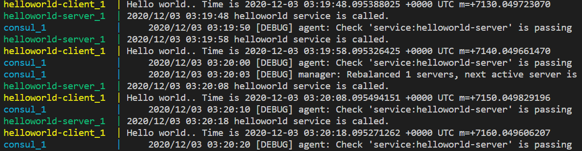
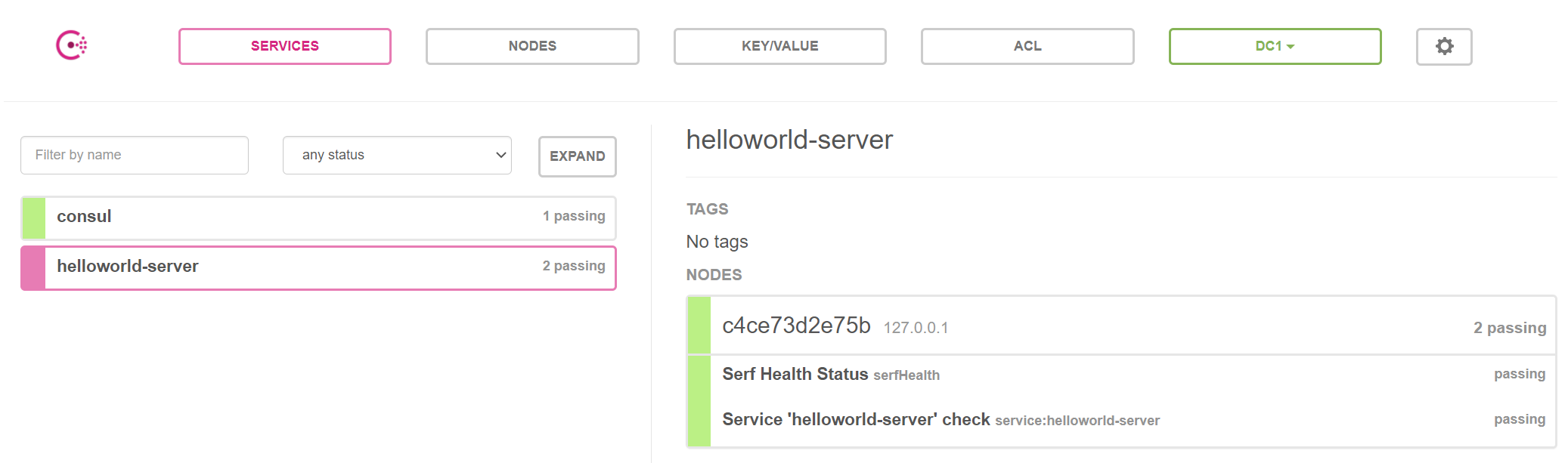
Everything is setted up, you can verify the result both in the terminal and Consul UI as following:

Introduction

This post will demonstrate how to do inter-thread communication in Golang concurrent programming. Generally speaking, there are two ways for this fundamental question: shared memory and message passing. You’ll see how to do these in Golang based on a case study and some tricky problems around it.

Background

Golang is a new popular and powerful programming language that aims to provide a simple, efficient, and safe way to build multi-threaded software.

Concurrent programming is one of Go’s main selling points. Go uses a concept called goroutine as its concurrency unit. Goroutine is a complex but interesting topic, you can find many articles about it online, This post will not cover concepts about it in detail. Simply speaking, goroutine is a user-space level thread which is lightweight and easy to create.

As mentioned above, one of the complicated problems when we do concurrent programming is that inter-thread (or inter-goroutine) communication is very error-prone. In Golang, it provides frameworks for both shared memory and message passing. However, it encourages the use of channels over shared memory.

You’ll see how both of these methods in Golang based on the following case.

Case study

The example is very simple: sums a collection (10 million) of integers. In fact this example is based on this good article. It used the shared memory way to realize the communication between goroutines. I expand this example and implemented the message passing way to show the difference.

Shared Memory

Go supports traditional shared memory accesses among goroutines. You can use various traditional synchronization primitives such as lock/unlock (Mutex), condition variable (Cond) and atomic read/write operations(atomic).

In the following implementation, you can see Go uses WaitGroup to allow multiple goroutines to do their tasks before a waiting goroutine. This usage is very similar to pthread_join in C.

Goroutines are added to a WaitGroup by calling Add method. And the goroutines in a WaitGroup call Done method to notify their completion, while a goroutine make a call to Wait method to wait for all goroutines’ completion.

1
2
3
4
5
6
7
8
9
10
11
12
13
14
15
16
17
18
19
20
21
22
23
24
25
26
27
28
29
30
31
32
33
34
35
36
37
38
39
40
41
42
43
44
45
46
47
48
49
50
51
52
53
54
55
56
57
58
59
60
61
62
63
64

package main

import (
	"fmt"
	"math/rand"
	"runtime"
	"sync"
	"sync/atomic"
)

func main() {
	numbers := generateList(1e7)

	fmt.Println("add: ", add(numbers))
	fmt.Println("add concurrent: ", addConcurrent(runtime.NumCPU(), numbers))
}

func generateList(totalNumbers int) []int {
	numbers := make([]int, totalNumbers)
	for i := 0; i < totalNumbers; i++ {
		numbers[i] = rand.Intn(totalNumbers)
	}
	return numbers
}

func add(numbers []int) int {
	var v int
	for _, n := range numbers {
		v += n
	}
	return v
}

func addConcurrent(goroutines int, numbers []int) int {
	var v int64
	totalNumbers := len(numbers)
	lastGoroutine := goroutines - 1

	strid := totalNumbers / goroutines

	var wg sync.WaitGroup
	wg.Add(goroutines)

	for g := 0; g < goroutines; g++ {
		go func(g int) {
			start := g * strid
			end := start + strid
			if g == lastGoroutine {
				end = totalNumbers
			}

			var lv int
			for _, n := range numbers[start:end] {
				lv += n
			}
			atomic.AddInt64(&v, int64(lv))
			wg.Done()
		}(g)
	}

	wg.Wait()
	return int(v)
}

In the example above the int64 variable v is shared across goroutines. When this variable needs to be updated, an atomic operation was done by calling atomic.AddInt64() method to avoid race condition and nondeterministic result.

That’s how shared memory across goroutines works in Golang. Let’s go to message passing way in next section.

Message Passing

In Golang world, there is one sentence is famous:

Don’t communicate by sharing memory; share memory by communicating

For that, Channel(chan) is introduced in Go as a new concurrency primitive to send data across goroutines. This is also the way Golang recommended you to follow.

So the concurrent program to sum 10 million integers based on Channel goes as below:

1
2
3
4
5
6
7
8
9
10
11
12
13
14
15
16
17
18
19
20
21
22
23
24
25
26
27
28
29
30
31
32
33
34
35
36
37
38
39
40
41
42
43
44
45
46
47
48
49
50
51
52
53

package main

import (
	"fmt"
	"math/rand"
	"runtime"
)

func main() {
	var result int64
	numbers := generateList(1e7)

	goroutines := runtime.NumCPU()
	lastGoroutine := goroutines - 1

	totalNumbers := len(numbers)
	strid := totalNumbers / goroutines

	c := make(chan int)

	for g := 0; g < goroutines; g++ {
		start := g * strid
		end := start + strid
		if g == lastGoroutine {
			end = totalNumbers
		}

		go add(numbers[start:end], c)
	}

	for l := range c {
		result += int64(l)
	}

	fmt.Println("add concurrent: ", result)
}

func generateList(totalNumbers int) []int {
	numbers := make([]int, totalNumbers)
	for i := 0; i < totalNumbers; i++ {
		numbers[i] = rand.Intn(totalNumbers)
	}
	return numbers
}

func add(numbers []int, c chan int) {
	var v int
	for _, n := range numbers {
		v += n
	}
	c <- v
}

To create a typed channel, you can call make method. In this case, since the value we need to pass is an integer, so we create an int type channel with c := make(chan int). To read and write data to that channel, you can use <- operator. For example, in the add goroutine, when we get the sum of integers, we use c <- v to send data to the channel.

To read data from the channel in the main goroutine, we use a build-in method range in Golang which can iterate through data structure like slice, map and channel.

That’s it. Simple and beautiful.

Hit the Deadlock

Let’s build and run the above solution. You’ll get an error message as following:

1

fatal error: all goroutines are asleep - deadlock!

The deadlock issue occurs because of these two reasons. Firstly by default sends and receives to a channel are blocking. When a data is send to a channel, the control in that goroutine is blocked at the send statement until some other Goroutine reads from the channel. Similarly when data is read from a channel, the read is blocked until some Goroutine writes data to that channel. Secondly, range only stops when the channel is closed. In this case, each add Goroutine send only one value to the channel but didn’t close the channel. And the main Goroutine keeps waiting for something to be written (in fact, it can read 4 values, but after that it doesn’t stop and keep waiting for more data). So all of the Goroutines are blocked and none of them can continue the execution. Then hit a deadlock.

Fix the Deadlock

1
2
3
4
5
6
7
8
9
10
11
12
13
14
15
16
17
18
19
20
21
22
23
24
25
26
27
28
29
30
31
32
33
34
35
36
37
38
39
40
41
42
43
44
45
46
47
48
49
50
51
52
53

package main

import (
	"fmt"
	"math/rand"
	"runtime"
)

func main() {
	var result int64
	numbers := generateList(1e7)

	goroutines := runtime.NumCPU()
	lastGoroutine := goroutines - 1

	totalNumbers := len(numbers)
	strid := totalNumbers / goroutines

	c := make(chan int)

	for g := 0; g < goroutines; g++ {
		start := g * strid
		end := start + strid
		if g == lastGoroutine {
			end = totalNumbers
		}

		go add(numbers[start:end], c)
	}

	for j := 0; j < goroutines; j++ {
		result += int64(<-c)
	}

	fmt.Println("add concurrent: ", result)
}

func generateList(totalNumbers int) []int {
	numbers := make([]int, totalNumbers)
	for i := 0; i < totalNumbers; i++ {
		numbers[i] = rand.Intn(totalNumbers)
	}
	return numbers
}

func add(numbers []int, c chan int) {
	var v int
	for _, n := range numbers {
		v += n
	}
	c <- v
}

Let use the manual for loop, in each iteration we read the value from the channel and sum together. Run it again. The deadlock is resolved.

Background

In this post, I want to introduce xv6 which is a “simple, Unix-like operating system”.

xv6 is not only an open-source project, but also it is used for teaching purposes in MIT’s Operating Systems Engineering(6.828) course as well as many other institutions.

If you’re like me, always want to learn operating system, I guess you’ll face a very steep learning curve since operating system is complex.

For learning purpose, we need an operating system project which is not too complex and not too simple. Luckily, xv6 is just for this purpose which is simple enough to follow up as an open source project, yet still contains the important concepts and organization of Unix.

Resource

Since xv6 is an open source project, you can easily find many resources online.

Personally I recommend to use this page, which is the latest teaching resource for the corresponding MIT course. You can find source code, examples, slides and videos there. Very helpful!

Environment setup for xv6 project

On the MIT course’s document, there are many solutions for setting up the xv6 development environment. You can follow those solutions, it will work.

For your convenience, I make a Dockerfile to build the docker image which contains all the necessary dependencies to keep working on xv6. The Dockerfile goes as following:

1
2
3
4
5
6
7
8
9
10
11
12
13
14
15

FROM ubuntu:latest

ARG DEBIAN_FRONTEND=noninteractive

RUN apt-get -qq update

RUN apt-get install -y git \
                    build-essential \
                    gdb-multiarch \
                    qemu-system-misc \
                    gcc-9-riscv64-linux-gnu \
                    gcc-riscv64-linux-gnu \
                    binutils-riscv64-linux-gnu\
                    tmux \
                    qemu

Table of Contents

First I have to admit that memory management is a big( and important) topic in operating system. This post can’t cover everything related to it.

In this post, I want to share something interesting I learned about stack memory management. Especially understand how the stack frame of function call works, which’s the most important part of stack memory. I will explain the mechanism in detail with examples and diagrams.

Briefly speaking, the contents of this post is:

• Memory layout of a process
• Stack memory contents
• CPU register related to stack memory management
• Stack frame of function call and return mechanism

To understand the concepts and machanisms deeply, a few assembly code will be shown in this post, you don’t have to know assembly lauguage as an expert for reading this post, I will add comments for these assembly codes to make explain what’s their functionalities.

Stack Memory Management Basic

Memory Layout of Process

Before we talk about Stack memory management, it’s necessary to understand memory layout of a process.

When you create a program, it is just some Bytes of data which is stored in the disk. When a program executes then it starts loading into memory and become a live entity. In a more specify way, some memory (virtual memory) is allocated to each process in execution for its usage by operating system. The memory assigned to a process is called process’s virtual address space( short for VAS). And memory layout use diagrams to help you understand the concept of process virtual address space easily.

There are some awesome posts on the internet about memory layout. And the most two critical sections are: Stack and Heap. Simply speaking, Stack is the memory area which is used by each process to store the local variables, passed arguments and other information when a function is called. This is the topic of this post, you’ll know more detailed in the following sections. While Heap segment is the one which is used for dynamic memory allocation, this is another more complex topic out of this post’s scope.

Stack Memory Basics

Stack Memory is just memory region in each process’s virtual address space where stack data structure (Last in, first out) is used to store the data. As we mentioned above, when a new function call is invoked, then a frame of data is pushed to stack memory and when the function call returns then the frame is removed from the stack memory. This is Stack Frame which represent a function call and its argument data. And every function has its own stack frame.

Let’s say in your program there are multiple functions call each other in order. For example, main() -> f1() -> f2() -> f3(), main function calls function one f1(), then function one calls function two f2(), finally function two calls function three f3(). So based on the Last in first out rule, the stack memory will be like as below:

Note: the top of the stack is the bottom part of the image. Don’t feel confused for that.

Stack memory contents

After understand stack frames, now let’s dive deep into each stack frame to discover its contents.

Each stack frame contains 4 parts:

• Parameter passed to the callee function
• Return address of the caller function
• Base pointer
• Local variables of the callee function

Caller and callee is very easy to understand. Let’s say main() -> f1(), then caller function is main() while callee function is f1(). Right?

For the above 4 four parts, there are something need to emphasis. Firstly the size of return address of the caller function is fixed, for example, in 32 bits system the size is 4B. And Base pointer size is fixed as well, it’s also 4B in a 32 bits system. This fixed size is important, you’ll see the reason in following sections.

Next, in the above diagram you see two kinds of pointers: base pointer and stack pointer. Let’s check them one by one.

Stack pointer: pointer to the top of the stack. When stack adds or removes data then stack pointer will change correspondingly. Stack pointer is straight forward and not difficult to understand, right?
Base pointer: is also called frame pointer which points to the current active frame. And the current active frame is the topmost frame of the stack.

The base pointer is conventionlly used to mark the start of a function’s stack frame, and the area of the stack managed by that function. As we mentioned above, since the size of return address and base pointer is fixed, so based on the address of base pointer you can get all the data in that stack frame. Local variables can be accessed with positive offset and passed parameters can be got with negative offset. That’s the reason why it is called base pointer. Great design, right?

The other thing need to discuss is what’t the content of base pointer part in each stack frame? In the above diagram you see that a 4 bytes data is pushed into the stack, we call it base pointer. But what’s the data? In fact, base pointer is designed to store the caller's base pointer address. This is also a smart design to make function return works well. We’ll discuss more about it later.

CPU register

To understand stack memory management, you’ll need to know 3 interesting CPU register:

• eip: Instruction pointer register which stores the address of the next instruction to be run.
• esp: Stack pointer register which stores the address of the top of the stack at any time.
• ebp: Base pointer register which stores base pointer address of callee’s stack frame. And the content at this address is the caller’s base pointer value (we already mentioned this point above).

Until now, you see all the necessary stuff: stack frame, stack frame content and CPU registers. Let’s see how they play together to make stack frames of function call and return works. You’ll see how this simple but beautiful design realizes such a complex task.

Mechanism of function call and return

In this section, you’ll understand how function call and return works by reading a few assembly codes (which are not difficult to understand).

function call

Step one: as you already see in the above diagram the first part of each stack frame is the passed parameters to the callee. So all the arguments are pushed on the stack as the following codes shows:

1
2

push arg2;
push arg1;

push is the assembly instruction to push data onto the stack. And usually the arguments are pushed to the stack in the reverse order that they’re declared in function.

Step two: the second part is the Return address of the caller fn, so we need to push the address of next instruction in caller function as Return address in callee’s stack frame. As we introduced in the last section, the address of next instruction will be stored in EIP register, right? The assembly code goes as following:

1

push eip;

Step three: upon entrying to the callee function, the old EBP value (the caller function’s base pointer address) is pushed onto the stack and then EBP is set to the value of ESP. Then the ESP is decremented (since the stack grows downward in stack memory) to allocate space for the local variables. And the codes goes as following:

1
2

push ebp;
mov ebp esp;

mov - the mov instruction copies the data item referred to by its second operand into the location referred to by its first operand.

So mov %ebp %esp just means set EBP a new value of ESP. Please note that, ESP value changes when data is pushed or popped onto/from the stack. But it’s always points to the top of the stack. Before this mov %ebp %esp instruction, ESP is pointing to the address just after the return address of the caller, and it should be the address of callee’s base pointer and just what EBP should store, this instruction makes sense, right?

From that on, during the execution of the callee function, the passed arguments to the function are located at the positive offsets from EBP, and the local variables are located at the negative offsets from EBP, you already see this conclusion above.

Inside a function, the stack would look like this:

1
2
3
4
5
6

| <argument 2>       |
| <argument 1>       |
| <return address>   |
| <old ebp>          | <= %ebp
| <local var 1>      |
| <local var 2>      | <= %esp

function return

Step one: upon exit from the callee function, all the function has to do is set ESP to the value of EBP. In this way can simply deallocates/releases the local variables from the stack. And then it can also expose callee’s base pointer on the top of the stack for next step operation.

1

mov esp, ebp;

This instruction is restoring the saved value of ESP upon entering the function, at that point what we did is mov ebp esp. Smart design, right?

Step two: since ESP already reset to the address of base pointer, next step we can simply pop the old EBP value from the top of stack as following:

1

pop ebp;

pop instruction retrieves the topmost value from the stack and puts the value into the second operand, in this case is EBP. Remember the callee function’s base pointer stores the caller function’s base pointer, so this simple pop ebp instruction realize EBP register restore perfactly. Great design, right?

Step three: next is straight forward, we need to pop the caller function return address to EIP.

1

pop eip;

Similar to step two, right? Now the system knows the next instruction (pointing to the return address in the caller function) need to run. The execution context is giving back to the caller function.

Upon returning back to the caller function, it can then increase ESP register again to remove the passed function arguments it pushed onto the stack. At this point, the stack frames becomes the same as it was in prior to invoking the callee function.

Why develop in Docker container?

Docker is the hottest technology to deploy and run the software. The key benefit of Docker is that it allows users to package an application with all of its dependencies into a standardized unit for software development. Compared with virtual machines, containers do not have high overhead and hence enable more efficient usage of the underlying system and resources.

Besides deploying and running applications, Docker containers can also make your local development work easier, especially when you need to set up a specific environment with many dependencies.

In my case, I have a project which is a C++ application running on the Linux platform. But on personal machines I’m running macOS and Windows systems, I didn’t install Linux platform on my computer. Before I start working on this project, I need to fix the platform/environment issue.

The first idea is, of course, using virtual-machines with VirtualBox and install the Linux system in it. This process will be time-consuming and tedious. So I decided to use Docker container to speed up the environment configuration step.

I will share the experience step by step. The whole process is lightweight and quick, also can practice your Docker related skills.

Create the Docker container

To build a Docker image, we need a Dockerfile, which is a text document(without a file extension) that contains the instructions to set up an environment for a Docker container. The Docker official site is the best place to understand those fundamental and important knowledge.

In my case the basic Dockerfile goes as following:

1
2
3
4
5
6
7
8
9
10
11
12
13
14
15
16

# Download base image ubuntu 20.04
FROM ubuntu:20.04

# Disable Prompt During Packages Installation
ARG DEBIAN_FRONTEND=noninteractive

# Update Ubuntu Software repository
RUN apt-get update && apt-get install -y \
    make \
    cmake \
    g++ \
    libncurses5-dev \
    libncursesw5-dev \
&& rm -rf /var/lib/apt/lists/*

CMD ["bash"]

FROM : the first part is the FROM command, which tells us what image to base this off of (as we know, Docker is following a multi-layer structure). In my case, it’s using the Ubuntu:20.04 image, which again references a Dockerfile to automate the process.

ARG: ARG instruction defines a variable that can be passed at build time to pass environment info. In this case, just to disable the console output during the following Linux package installation process.

RUN: the next set of calls are the RUN commands. This RUN instruction allows you to install your application and packages for it. RUN executes commands in a new layer and creates a new layer by committing the results. Usually, you can find several RUN instructions in a Dockerfile. In this case, I want to install the C++ compiler and build tools (and some other specific dependency packages for development) which is not available in the Ubuntu base image.

CMD: the last instruction CMD allows you to set a default command, which will be executed when you run the container without specifying a command. If Docker container runs with a command, this default one will be ignored.

With this Dockerfile, we can build the image with the next Docker command:

1

docker build -t linux-cpp .

This will build the desired Docker image tagged as linux-cpp. You can list(find) this new image in your system with command docker images:

1
2

REPOSITORY          TAG                 IMAGE ID            CREATED             SIZE
linux-cpp           latest              5463808c4488        8 days ago          320MB

Now you can run the docker container with the newly build linux-cpp image:

1

docker run -it --name cpp-dev --rm linux-cpp

Mount source code into container

Follow the above steps, you can have a running Docker container with C++ development dependencies in Linux environment.

Next, you can directly start your C++ program inside the container, then build and run your code.

But if you just put your program inside the container, you will have a high risk to lose your code when the container is deleted.

The better way is placing your program source code on your local machine and sync the codes into the container as you program. This is where mount can help you. Mount and Volume is an important topic for Docker, you can find some posts for deeper introduction.

In my case, I can realize my target with the following command:

1

docker run -it --name cpp-dev  --rm  -v ${PWD}:/develop  linux-cpp

the key and interesting part is: -v ${PWD}:/develop, this will mount the current directory of the host machine into the develop directory inside the container. If develop directory is not there, Docker will make it for you.

Note: the current directory pwd command’s usage has some variants based on your host machine. The above command works for the Powershell of Windows, if you are using git bash on Windows, please try:

1

-v /$(pwd):/develop

For Mac users, try the following:

1

-v $(pwd):/develop

Now you can happily code your program in your familiar host machine, save the code change and sync them into the container. Then build and run your code inside the container with every dependency it needs.

Background

Selector is an essential part of the entire NgRx state management system, which is much more complicated than the action and reducer part based on my learning and development experience. Sometimes I feel it is like a black box, which hides many excellent designs and techniques. I spend some time and dig into the source code of NgRx to take a look at the internals of the black box. This post (and later posts) will share some interesting points I found during the process.

When using NgRx, developers always do something like this:

1
2
3
4

export const animalListState: MemoizedSelector<State, Animal[]> = createSelector(
  rootState,
  (state: RootState): AnimalListState => state.animalList
);

createSelector method return a selector function, which can be passed into the store.select() method to get the desired state out of the store.

By default, the type of the returned function from createSelector is MemoizedSelector<State, Result>. Have you ever notice that? This post will introduce what it is and how it works.

What is memoization?

Memoization is a general concept in computer science. Wikipedia explains it as follows:

In computing, memoization or memoisation is an optimization technique used primarily to speed up computer programs by storing the results of expensive function calls and returning the cached result when the same inputs occur again.

You can find many articles online for explaining memoization with code examples. Simply speaking, a hash map is used for the cached result. Technically it’s not difficult at all.

Memoization is a great optimization solution of pure function. Generally speaking, A pure function is a function where the return value is only determined by its input values, without side effects.

As you may know, Selector is a pure function. memoizedSelector is just a normal selector function with memoization optimization. Next, let’s see how it works in the design of the NgRx library.

Source code of memoizedSelector

In the source code of NgRx, you can find the selector related code in the path of platform/modules/store/src/selector.ts.

selector.ts file is roughly 700 lines, which hold all the functionalities of it. There are many interesting points inside this module, which I can share in another article, but this post focus on memoization. So I pick up all the necessary code and put it as follows:

1
2
3
4
5
6
7
8
9
10
11
12
13
14
15
16
17
18
19
20
21
22
23
24
25
26
27
28
29
30
31
32
33
34
35
36
37
38
39
40
41
42
43
44
45
46
47
48
49
50
51
52
53
54
55
56
57
58
59
60
61
62
63
64
65
66
67
68
69
70
71

export type AnyFn = (...args: any[]) => any;

export type ComparatorFn = (a: any, b: any) => boolean;

export type MemoizedProjection = {
    memoized: AnyFn;
    reset: () => void;
    setResult: (result?: any) => void;
};

export function isEqualCheck(a: any, b: any): boolean {
    return a === b;
};

function isArgumentsChanged(
    args: IArguments,
    lastArguments:IArguments,
    comparator: ComparatorFn
) {
    for (let i = 0; i < args.length ; i++) {
        if (!comparator(args[i], lastArguments[i])) {
            return true;
        }
    }
    return false;
}

export function defaultMemoize(
    projectionFn: AnyFn,
    isArgumentsEuqal = isEqualCheck,
    isResultEqual = isEqualCheck
): MemoizedProjection {
    let lastArguments: null | IArguments = null;
    let lastResult: any = null;
    let overrideResult: any;

    function reset() {
        lastArguments = null;
        lastResult = null;
    }

    function setResult(result: any = undefined) {
        overrideResult = result;
    }

    function memoized(): any {
        if (overrideResult !== undefined) {
            return overrideResult;
        } 
        if (!lastArguments) {
            lastResult = projectionFn.apply(null, arguments as any);
            lastArguments = arguments;
            return lastResult;
        }

        if (!isArgumentsChanged(arguments, lastArguments, isArgumentsEuqal)) {
            return lastResult;
        }

        const newResult = projectionFn.apply(null, arguments as any);
        lastArguments = arguments;

        if (isResultEqual(lastResult, newResult)) {
            return lastResult;
        }

        lastResult = newResult;
        return newResult;
    }
    return { memoized, reset, setResult};
}

There are many interesting Typescript stuff in the above code block. But for memoization, you can focus on the method defaultMemoize. In the following section, I will show you how it can make your program run faster.

Explore the memoizedSelector method

To show how memoization works, I create a simple method slowFunction as following, to simulate that a method running very slowly:

1
2
3
4
5
6
7
8
9
10

export function slowFunction(val: number): number {
    const pre = new Date();
    while (true) {
        const now = new Date();
        if (now.valueOf() - pre.valueOf() > 2000) {
            break;
        }
    }
    return val;
}

And then test it with the following scripts:

1
2
3
4
5
6
7
8
9
10
11
12
13
14
15
16
17
18
19
20
21
22
23
24

import { defaultMemoize } from "./memoizedSelector";
import { slowFunction } from "./slowFunction";

// run slowFunction without memoization
console.log("First call of slowFunction(2)");
let pre = new Date();
slowFunction(2);
console.log("It takes" + ((new Date()).valueOf() - pre.valueOf())/1000 +  "seconds \n");
console.log("Second call of slowFunction(2)");
pre = new Date();
slowFunction(2);
console.log("It takes" + ((new Date()).valueOf() - pre.valueOf())/1000 +  "seconds \n");

// run slowFunction with memoization

const fastFunction = defaultMemoize(slowFunction);
console.log("First call of fastFunction(2)");
pre = new Date();
fastFunction.memoized(2);
console.log("It takes" + ((new Date()).valueOf() - pre.valueOf())/1000 +  "seconds \n");
console.log("Second call of fastFunction(2)");
pre = new Date();
fastFunction.memoized(2);
console.log("It takes" + ((new Date()).valueOf() - pre.valueOf())/1000 +  "seconds \n");

The output goes as folllowing:

1
2
3
4
5
6
7
8
9
10
11
12

$ ts-node index.ts
First call of slowFunction(2)
It takes2.001seconds

Second call of slowFunction(2)
It takes2.001seconds

First call of fastFunction(2)
It takes2.002seconds

Second call of fastFunction(2)
It takes0.001seconds

Compared with the original slowFunction method, the memoized method fastFunction can directly output the result for the same input. That’s the power of memoization, hope you can master it.

What’s Marble Testing

RxJS is a powerful tool to handle various asynchronous tasks. Sometime RxJS observables are hard to test. In the community, there is one particular unit testing solution for RxJS observables called marble testing.

For marble testing, you can refer to these articles. They all do an excellent job of introducing what it is.

A real case to show Marble Testing’s power

Recently in my development work, I came across a case where I used marble testing properly to solve the issue.

The background is for my application in the root index.html file, there is one third-party javascript library/SDK. For some business reasons, after the third-party library is loaded, we bind some value to the global window object.

1
2
3

window.onSecretLibraryLoad = (res) => {
  window.SecretLibrary = res; 
};

Before the loaded event is triggered, the window.SecretLibary was undefiend. After the event is triggered, it will be assigned some value.

This global value is vital for my application since one of the UI components depends on it to determine to show or hide.

Since the script was loaded with async flag for performance consideration, this component needs to check the window.SecretLibrary value repeatedly.

1
2
3
4
5
6
7
8
9
10
11
12
13
14
15
16
17
18
19
20

export class UIComponent implements OnInit {
    public isSecretLibraryReady$: Observable<boolean>;
    public ngOnInit(): void {
        this.isSecretLibraryReady$ = this.getSecretLibraryLoadStatus();
    }

    public getSecretLibraryLoadStatus(): Observable<boolean> {
        return timer(0, 500).pipe(
            map((t) => ({
                currentTimeTick: t,
                isReady: Boolean((window as any).SecretLibrary)
            })),
            takeWhile(
                (val) => !val.isReady && val.currentTimeTick <= 30000/500,
                true
            ),
            pluck("isReady")
        );
    }
}

The interesting part comes from the getSecretLibraryLoadStatus function. It utilizes the timer, map, takeWhile, and pluck operators of RxJS library to realize the repeatedly status checking and updating purpose.

RxJS operator is not this article’s topic, so I will not dig deep into it. Just add one comment for the takeWhile part, which seems a little hard to understand at the first look. It defines two conditions to stop the observable: first case is the window.SecretLibrary value is not undefined, which means the script is loaded; the second case is it reaches the maximum time limit (30 seconds).

How to test it: marble testing

Traditionally we use subscribe and assert pattern to test RxJS observables. But for the case, as mentioned above: time-based observables, the traditional solution can’t handle it well. We can’t wait 30 seconds when we run the unit tests during local development or in CI pipeline. That’s unacceptable.

Marble testing can fix this issue correctly by the concept of virtual time. For what is virtual time, you can refer to these great articles. I will not discuss it at a detailed level in this post. Simply speaking, virtual time empowers us to test asynchronous RxJS observable synchronously. In virtual time asynchronous functions like setTimeout and setInterval will use fake time instead of actual time. And the magic comes from the TestScheduler of RxJS.

The marble testing solution as following:

1
2
3
4
5
6
7
8
9
10
11
12
13
14
15
16
17
18
19
20
21
22
23
24
25
26
27
28
29
30
31
32
33
34
35
36
37
38

describe("UIComponent", () => {
  let component: UIComponent;
  let fixture: ComponentFixture<UIComponent>;
  let scheduler: TestScheduler;

  beforeEach(async(() => {
    TestBed.configureTestingModule({
      declarations: [UIComponent],
    }).compileComponents();
  }));

  beforeEach(() => {
    fixture = TestBed.createComponent(UIComponent);
    component = fixture.componentInstance;
    scheduler = new TestScheduler((actual, expected) => expect(actual).toEqual(expected));
    (window as any).SecretLibrary = undefined;
  });

  it("getSecretLibraryLoadStatus method should return a boolean observable stream, for script load success case", () => {
    scheduler.run(({ expectObservable }) => {
      timer(2 * 1000).subscribe(() => {
        (window as any).SecretLibrary = "SecretLibrary";
      });
      // tricky point about marble test: a, b, c these placeholders account 1 frame of virtual time
      expectObservable(component.getSecretLibraryLoadStatus()).toBe(
        "a 499ms b 499ms c 499ms d 499ms (e|)",
        {
          a: false,
          b: false,
          c: false,
          d: false,
          e: true
        }
      );
    });
  });
});

Let me emphasize several key points to understand the above testing case. getSecretLibraryLoadStatus will repeatedly check the status of window.SecretLibrary every 500 milliseconds and return a boolean value stream.

I manually set the window.SecretLibrary value after 2 seconds by calling this:

1
2
3

timer(2 * 1000).subscribe(() => {
  (window as any).SecretLibrary = "SecretLibrary";
});

So Let’s imagine what the result should be: the first four emit value will be false, and the last value is true. That’s the expected observable.

But please notice that scheduler.run, everything run inside the callback will use virtual time. So we didn’t wait 2 seconds for the timer operator. Instead, it runs synchronously.

The second point needs to notice is the syntax of the marble string a 499ms b 499ms c 499ms d 499ms (e|). Yes, it looks a little wired, but be careful that’s the correct way to represent marble. The alphanumeric values represent an actual emitted value, which advances time one virtual frame.

Here I only show the case where the third-party script load successfully. Of course, to have full testing coverage, we need to consider the negative case where the script failed to load. You can figure it out.

Summary

In this post, I didn’t go into the detailed syntax of marble testing. I think the reader can find the related document easily. I record a real usage case in the development where marble testing can show its power to handle async observables.

Part 2

Circular List

Judge a linked list is circular or not

1
2
3
4
5
6
7
8
9
10
11
12
13
14
15

function circular(list) {
  let slow = list.getFirst();
  let fast = list.getFirst();

  while (fast.next && fast.next.next) {
    slow = slow.next;
    fast = fast.next.next;

    if (slow === fast) {
      return true;
    }
  }

  return false;
}

Tree

1
2
3
4
5
6
7
8
9
10
11
12
13
14
15
16
17
18
19
20
21
22
23
24
25
26
27
28
29
30
31
32
33
34
35
36
37
38
39
40
41
42
43
44
45
46
47

class Node {
  constructor(data) {
    this.data = data;
    this.children = [];
  }

  add(data) {
    this.children.push(new Node(data));
  }

  remove(data) {
    this.children = this.children.filter(node => {
      return node.data !== data;
    });
  }
}

class Tree {
  constructor() {
    this.root = null;
  }
  // 广度优先
  traverseBF(fn) {
    // 初始化一个数组
    const arr = [this.root];
    // 循环判断
    while (arr.length) {
      // 取得头部的元素
      const node = arr.shift();
      // 把头部元素的children push到array里
      arr.push(...node.children);
      fn(node);
    }
  }
  // 深度优先
  traverseDF(fn) {
    const arr = [this.root];
    while (arr.length) {
      const node = arr.shift();

      arr.unshift(...node.children);
      fn(node);
    }
  }
}

module.exports = { Tree, Node };

Tree level width

1
2
3
4
5
6
7
8
9
10
11
12

Given the root node of a tree, return
an array where each element is the width
of the tree at each level.
--- Example
Given:
    0
  / |  \
1   2   3
|       |
4       5
Answer: [1, 3, 2]

solution:

1
2
3
4
5
6
7
8
9
10
11
12
13
14
15
16
17
18

function levelWidth(root) {
  const arr = [root, 's'];
  const counters = [0];

  while (arr.length > 1) {
    const node = arr.shift();

    if (node === 's') {
      counters.push(0);
      arr.push('s');
    } else {
      arr.push(...node.children);
      counters[counters.length - 1]++;
    }
  }

  return counters;
}

Events

1
2
3
4
5
6
7
8
9
10
11
12
13
14
15
16
17
18
19
20
21
22
23
24
25
26
27
28
29
30
31
32
33
34
35

// --- Directions
// Create an 'eventing' library out of the
// Events class.  The Events class should
// have methods 'on', 'trigger', and 'off'.

class Events {
  constructor() {
    this.events = {};
  }

  // Register an event handler
  on(eventName, callback) {
    if (this.events[eventName]) {
      this.events[eventName].push(callback);
    } else {
      this.events[eventName] = [callback];
    }
  }

  // Trigger all callbacks associated
  // with a given eventName
  trigger(eventName) {
    if (this.events[eventName]) {
      for (let cb of this.events[eventName]) {
        cb();
      }
    }
  }

  // Remove all event handlers associated
  // with the given eventName
  off(eventName) {
    delete this.events[eventName];
  }
}

Binary Search Tree

1
2
3
4
5
6
7
8
9
10
11
12
13
14
15
16
17
18
19
20
21
22
23
24
25
26
27
28
29
30
31
32
33
34
35
36
37
38
39
40
41
42
43
44
45
46
47
48
49
50
51
52
53

// 1) Implement the Node class to create
// a binary search tree.  The constructor
// should initialize values 'data', 'left',
// and 'right'.
// 2) Implement the 'insert' method for the
// Node class.  Insert should accept an argument
// 'data', then create an insert a new node
// at the appropriate location in the tree.
// 3) Implement the 'contains' method for the Node
// class.  Contains should accept a 'data' argument
// and return the Node in the tree with the same value.
// If the value isn't in the tree return null.

class Node {
  constructor(data) {
    // 每个node三个属性
    this.data = data;
    this.left = null;
    this.right = null;
  }

  insert(data) {
    if (data < this.data && this.left) {
      //对left子节点的递归insert
      this.left.insert(data);
    } else if (data < this.data) {
      // 赋值给left子节点
      this.left = new Node(data);
    } else if (data > this.data && this.right) {
      //对right子节点的递归insert
      this.right.insert(data);
    } else if (data > this.data) {
      // 赋值给right子节点
      this.right = new Node(data);
    }
  }

  contains(data) {
    if (this.data === data) {
      return this;
    }

    if (this.data < data && this.right) {
      // right子节点的contains操作
      return this.right.contains(data);
    } else if (this.data > data && this.left) {
      // left子节点的contains操作
      return this.left.contains(data);
    }

    return null;
  }
}

Validate the Binary Search Tree

1
2
3
4
5
6
7
8
9
10
11
12
13
14
15
16
17
18
19

function validate(node, min = null, max = null) {
  if (max !== null && node.data > max) {
    return false;
  }

  if (min !== null && node.data < min) {
    return false;
  }

  if (node.left && !validate(node.left, min, node.data)) {
    return false;
  }

  if (node.right && !validate(node.right, node.data, max)) {
    return false;
  }

  return true;
}

BubbleSort

1
2
3
4
5
6
7
8
9
10
11
12
13
14
15

function bubbleSort(arr) {
  // Implement bubblesort
  for (let i = 0; i < arr.length; i++) {
    for (let j = 0; j < (arr.length - i - 1); j++) {
      if (arr[j] > arr[j+1]) {
        const lesser = arr[j+1];
        arr[j+1] = arr[j];
        arr[j] = lesser;
      }
    }
  }

  // return the sorted array
  return arr;
}

Selection Sort

1
2
3
4
5
6
7
8
9
10
11
12
13
14
15
16
17
18
19

function selectionSort(arr) {
  for (let i = 0; i < arr.length; i++) {
    let indexOfMin = i;

    for (let j = i+1; j <arr.length; j++) {
      if (arr[j] < arr[indexOfMin]) {
        indexOfMin = j;
      }
    }

    if (indexOfMin !== i) {
      let lesser = arr[indexOfMin];
      arr[indexOfMin] = arr[i];
      arr[i] = lesser;
    }
  }

  return arr;
}

Merge Sort

1
2
3
4
5
6
7
8
9
10
11
12
13
14
15
16
17
18
19
20
21
22
23
24
25
26

function mergeSort(arr) {
  if (arr.length === 1) {
    return arr;
  }

  const center = Math.floor(arr.length / 2);
  const left = arr.slice(0, center);
  const right = arr.slice(center);
  // 神奇的递归
  return merge(mergeSort(left), mergeSort(right));
}

// 辅助函数merge，能够把两个已经排序的left和right数组，整合排序为一个array
function merge(left, right) {
  const results = [];

  while (left.length && right.length) {
    if (left[0] < right[0]) {
      results.push(left.shift());
    } else {
      results.push(right.shift());
    }
  }
  // 到这行的时候，left和right，至少有一个是空的了，所以不用纠结left和right的前后位置了。
  return [...results, ...left, ...right];
}

binary Gap

A binary gap within a positive integer N is any maximal sequence of consecutive zeros that is surrounded by ones at both ends in the binary representation of N.

For example, number 9 has binary representation 1001 and contains a binary gap of length 2. The number 529 has binary representation 1000010001 and contains two binary gaps: one of length 4 and one of length 3. The number 20 has binary representation 10100 and contains one binary gap of length 1. The number 15 has binary representation 1111 and has no binary gaps. The number 32 has binary representation 100000 and has no binary gaps.

1
2
3
4
5
6
7
8
9
10
11
12
13
14
15
16
17
18

function binaryGap(num) {
  let str = num.toString(2).split('')
  console.log(str)
  let counter = 0;
  let max = 0;
  str.forEach((char) =>  {
    if (char === '0') {
      counter ++;
    } else {
      if (counter > max) {
        max = counter;
      }
      counter = 0;
    }
    // console.log(counter)
  });
  return max;
}

Bug and Sell Stock

You will be given a list of stock prices for a given day and your goal is to return the maximum profit that could have been made by buying a stock at the given price and then selling the stock later on. For example if the input is: [45, 24, 35, 31, 40, 38, 11] then your program should return 16 because if you bought the stock at $24 and sold it at $40, a profit of $16 was made and this is the largest profit that could be made. If no profit could have been made, return -1.

1
2
3
4
5
6
7
8
9
10
11
12
13
14
15
16
17
18
19
20
21
22
23
24
25
26
27
28

function getMaxProfit(arr) {
  var minIdx = 0;
    var maxIdx = 1;
    var currMin = 0;
    var maxProfit = 0;

    if(arr.length < 2) {
        throw new Error("Need atleast two time periods to be profitable!");
    }

    for(var i = 1; i < arr.length; i++) {

        // new current min.
        if(arr[i] < arr[currMin]) {
          currMin = i;
        }

        // new best profit
        if(arr[maxIdx] - arr[minIdx] < arr[i] - arr[currMin]) {
                maxIdx = i;
              minIdx = currMin;
        }

    }

    maxProfit  = arr[maxIdx] - arr[minIdx];
    return maxProfit;
}

The Coding Interview Bootcamp: Data structure and algorithm.

Part 1

String Reverse

1
2
3

function reverse(str) {
  return str.split('').reduce((rev, char) => char + rev, '');
}

Paldinromes

1
2
3
4
5

function palindrome(str) {
  return str.split('').every((char, i) => {
    return char === str[str.length - i - 1];
  });
}

another way is based on recursive method:

1
2
3
4
5
6
7
8
9
10
11

function palindromeRecursive(str) {
  if (str.length <= 1) {
    return true;
  } else {
    if (str[0] !== str[str.length - 1]) {
      return false;
    } else {
      return palindromeRecursive(str.substring(1, str.length - 1))
    }
  }
}

Longest Paldinromes substring

1
2
3
4
5
6
7
8
9
10
11
12
13
14
15
16
17
18
19
20
21
22
23
24
25
26
27
28
29
30
31
32
33
34
35
36
37
38
39

function longestPalin(str) {
  str = treatStr(str);
  console.log(str)
  let max =  0;
  for (let i  = 1; i < str.length - 1; i++) {
    let radius = Math.min (i, str.length - i - 1);
    console.log(radius)
    let currentMax = getMaxSubLength(str, i, radius);
    if (max < currentMax) {
      max = currentMax + 1;
    }
  }
  return max;
}

function getMaxSubLength(str, i, radius) {
  let max = 0;
  for (let j = 0; j <= radius; j++) {
    if (str[i - j] === str[i + j]) {
      max = j;
    } else {
      break;
    }
  }
  return max;
}

function treatStr(str) {
  let rtn = '';
  for (let i = 0; i < str.length; i++) {
    if (i === str.length - 1) {
      rtn = rtn + str[i];
    } else  {
      rtn = rtn + str[i] + '#';
    }

  }
  return rtn;
}

Integer Reversal

1
2
3
4
5
6
7
8
9
10
11
12
13
14
15
16
17
18
19

// --- Directions
// Given an integer, return an integer that is the reverse
// ordering of numbers.
// --- Examples
//   reverseInt(15) === 51
//   reverseInt(981) === 189
//   reverseInt(500) === 5
//   reverseInt(-15) === -51
//   reverseInt(-90) === -9

function reverseInt(n) {
  const reversed = n
    .toString()
    .split('')
    .reverse()
    .join('');

  return parseInt(reversed) * Math.sign(n);
}

Anagrams

method1

1
2
3
4
5
6
7
8
9
10
11
12
13
14
15
16
17
18
19
20
21
22
23
24
25
26

function anagrams(stringA, stringB) {
  const aCharMap = buildCharMap(stringA);
  const bCharMap = buildCharMap(stringB);

  if (Object.keys(aCharMap).length !== Object.keys(bCharMap).length) {
    return false;
  }

  for (let char in aCharMap) {
    if (aCharMap[char] !== bCharMap[char]) {
      return false;
    }
  }

  return true;
}

function buildCharMap(str) {
  const charMap = {};

  for (let char of str.replace(/[^\w]/g, '').toLowerCase()) {
    charMap[char] = charMap[char] + 1 || 1;
  }

  return charMap;
}

method2

1
2
3
4
5
6
7
8
9
10
11
12

function anagrams(stringA, stringB) {
  return cleanString(stringA) === cleanString(stringB);
}

function cleanString(str) {
  return str
    .replace(/[^\w]/g, '')
    .toLowerCase()
    .split('')
    .sort()
    .join('');
}

Printing Steps

The effect we need is as following:

1
2
3
4
5
6
7
8
9
10
11
12
13

--- Examples
  steps(2)
      '# '
      '##'
  steps(3)
      '#  '
      '## '
      '###'
  steps(4)
      '#   '
      '##  '
      '### '
      '####'

solution based on recursive methods

1
2
3
4
5
6
7
8
9
10
11
12
13

function steps(n, row = 0, stair = '') {
  if (n === row) {
    return;
  }

  if (n === stair.length) {
    console.log(stair);
    return steps(n, row + 1);
  }

  const add = stair.length <= row ? '#' : ' ';
  steps(n, row, stair + add);
}

Enter the Matrix Spiral

The requirement goes as following:

1
2
3
4
5
6
7
8
9
10
11
12
13

--- Examples
  matrix(2)
    [[undefined, undefined],
    [undefined, undefined]]
  matrix(3)
    [[1, 2, 3],
    [8, 9, 4],
    [7, 6, 5]]
 matrix(4)
    [[1,   2,  3, 4],
    [12, 13, 14, 5],
    [11, 16, 15, 6],
    [10,  9,  8, 7]]

solution:

1
2
3
4
5
6
7
8
9
10
11
12
13
14
15
16
17
18
19
20
21
22
23
24
25
26
27
28
29
30
31
32
33
34
35
36
37
38
39
40
41
42
43
44

function matrix(n) {
  const results = [];

  for (let i = 0; i < n; i++) {
    results.push([]);
  }

  let counter = 1;
  let startColumn = 0;
  let endColumn = n - 1;
  let startRow = 0;
  let endRow = n - 1;
  while (startColumn <= endColumn && startRow <= endRow) {
    // Top row
    for (let i = startColumn; i <= endColumn; i++) {
      results[startRow][i] = counter;
      counter++;
    }
    startRow++;

    // Right column
    for (let i = startRow; i <= endRow; i++) {
      results[i][endColumn] = counter;
      counter++;
    }
    endColumn--;

    // Bottom row
    for (let i = endColumn; i >= startColumn; i--) {
      results[endRow][i] = counter;
      counter++;
    }
    endRow--;

    // start column
    for (let i = endRow; i >= startRow; i--) {
      results[i][startColumn] = counter;
      counter++;
    }
    startColumn++;
  }

  return results;
}

Fibonacci

solution based on memoization and recursive.

1
2
3
4
5
6
7
8
9
10
11
12
13
14
15
16
17
18
19
20
21
22
23

function memoize(fn) {
  const cache = {};
  return function(...args) {
    if (cache[args]) {
      return cache[args];
    }

    const result = fn.apply(this, args);
    cache[args] = result;

    return result;
  };
}

function slowFib(n) {
  if (n < 2) {
    return n;
  }

  return fib(n - 1) + fib(n - 2);
}

const fib = memoize(slowFib);

The most simplified method goes as following:

1
2
3
4
5
6
7
8
9
10
11
12

function memoize(fn) {
  const cache = {};
  return function(n) {
    if(cache[n]) {
      return cache[n];
    }
    const result = fn(n);
    cache[n] = result;

    return result;
  }
}

Make it more abstract like below:

1
2
3
4
5
6
7
8
9
10
11
12
13

function memoize(fn) {
  const cache = {};
  return function(...args) {
    if (cache[args]) {
      return cache[args];
    }

    const result = fn.apply(this, args);
    cache[args] = result;

    return result;
  };
}

Queue and Stack

1
2
3
4
5
6
7
8
9
10
11
12
13
14
15
16
17
18
19
20
21
22
23
24
25
26
27
28
29
30
31
32
33
34
35
36
37
38
39
40
41
42
43
44
45
46
47
48
49
50
51
52
53
54
55
56
57
58
59
60
61
62
63
64
65
66
67
68
69
70
71
72
73
74
75
76
77
78

class Queue {
  constructor() {
    this.data = [];
  }

  add(record) {
    this.data.unshift(record);
  }

  remove() {
    return this.data.pop();
  }
}

class Stack {
  constructor() {
    this.data = [];
  }

  push(record) {
    this.data.push(record);
  }

  pop() {
    return this.data.pop();
  }

  peek() {
    return this.data[this.data.length - 1];
  }
}
``` 

### Two Become One 

Implement a Queue data structure using two stacks

``` javascript
const Stack = require('./stack');

class Queue {
  constructor() {
    this.first = new Stack();
    this.second = new Stack();
  }

  add(record) {
    this.first.push(record);
  }

  remove() {
    while (this.first.peek()) {
      this.second.push(this.first.pop());
    }

    const record = this.second.pop();

    while (this.second.peek()) {
      this.first.push(this.second.pop());
    }

    return record;
  }

  peek() {
    while (this.first.peek()) {
      this.second.push(this.first.pop());
    }

    const record = this.second.peek();

    while (this.second.peek()) {
      this.first.push(this.second.pop());
    }

    return record;
  }
}

Linked List

1
2
3
4
5
6
7
8
9
10
11
12
13
14
15
16
17
18
19
20
21
22
23
24
25
26
27
28
29
30
31
32
33
34
35
36
37
38
39
40
41
42
43
44
45
46
47
48
49
50
51
52
53
54
55
56
57
58
59
60
61
62
63
64
65
66
67
68
69
70
71
72
73
74
75
76
77
78
79
80
81
82
83
84
85
86
87
88
89
90
91
92
93
94
95
96
97
98
99
100
101
102
103
104
105
106
107
108
109
110
111
112
113
114
115
116
117
118
119
120
121
122
123
124
125
126
127
128
129
130
131
132
133
134
135
136
137
138
139
140
141
142
143
144
145
146
147
148
149
150
151
152
153
154

class Node {
  constructor(data, next = null) {
    this.data = data;
    this.next = next;
  }
}

class LinkedList {
  constructor() {
    this.head = null;
  }

  insertFirst(data) {
    this.head = new Node(data, this.head);
  }

  size() {
    let counter = 0;
    let node = this.head;

    while (node) {
      counter++;
      node = node.next;
    }

    return counter;
  }

  getFirst() {
    return this.head;
  }

  getLast() {
    if (!this.head) {
      return null;
    }

    let node = this.head;
    while (node) {
      if (!node.next) {
        return node;
      }
      node = node.next;
    }
  }

  clear() {
    this.head = null;
  }

  removeFirst() {
    if (!this.head) {
      return;
    }

    this.head = this.head.next;
  }

  removeLast() {
    if (!this.head) {
      return;
    }

    if (!this.head.next) {
      this.head = null;
      return;
    }

    let previous = this.head;
    let node = this.head.next;
    while (node.next) {
      previous = node;
      node = node.next;
    }
    previous.next = null;
  }

  insertLast(data) {
    const last = this.getLast();

    if (last) {
      // There are some existing nodes in our chain
      last.next = new Node(data);
    } else {
      // The chain is empty!
      this.head = new Node(data);
    }
  }

  getAt(index) {
    let counter = 0;
    let node = this.head;
    while (node) {
      if (counter === index) {
        return node;
      }

      counter++;
      node = node.next;
    }
    return null;
  }

  removeAt(index) {
    if (!this.head) {
      return;
    }

    if (index === 0) {
      this.head = this.head.next;
      return;
    }

    const previous = this.getAt(index - 1);
    if (!previous || !previous.next) {
      return;
    }
    previous.next = previous.next.next;
  }

  insertAt(data, index) {
    if (!this.head) {
      this.head = new Node(data);
      return;
    }

    if (index === 0) {
      this.head = new Node(data, this.head);
      return;
    }

    const previous = this.getAt(index - 1) || this.getLast();
    const node = new Node(data, previous.next);
    previous.next = node;
  }

  forEach(fn) {
    let node = this.head;
    let counter = 0;
    while (node) {
      fn(node, counter);
      node = node.next;
      counter++;
    }
  }

  *[Symbol.iterator]() {
    let node = this.head;
    while (node) {
      yield node;
      node = node.next;
    }
  }
}